101. Least Squares Learning in Self-Referential Models#
101.1. Overview#
This lecture is a companion to Rational Learning and Rational Expectations, which presents the Bray-Kreps perspective on rational learning.
We examine the related but distinct question of whether least squares learning converges to a rational expectations equilibrium in self-referential models.
We present the framework of Marcet and Sargent [1989] for studying least squares learning in a class of self-referential linear stochastic models.
A self-referential model is one where the actual law of motion for the economy depends on the perceived law of motion of agents within it.
In a rational expectations equilibrium (REE) the two coincide: the perceived and actual laws of motion are the same.
But if agents start away from equilibrium and update their beliefs by running least squares regressions, will they converge to the REE?
Marcet and Sargent [1989] answer this question by using a powerful technique from systems-control engineering: the differential equation approach of Ljung [1977].
The key insight is that the stochastic difference equation of belief evolution can be approximated by a deterministic ordinary differential equation (ODE) in the limit.
Almost-sure convergence can be studied through the stability of that ODE.
Local stability of the small ODE is closely related to local convergence, while global almost-sure convergence also requires boundedness and domain-of-attraction conditions.
The framework unifies and extends earlier work by Bray [1982] and Bray and Savin [1986] and connects naturally to the distinction between learning within a rational expectations equilibrium (Bayesian updating inside a correctly specified model) and learning about one (adapting an OLS estimator whose data-generating process shifts with beliefs) discussed in Bray and Kreps [1987].
Let’s begin with the imports we’ll use throughout.
import numpy as np
import matplotlib.pyplot as plt
from numpy import linalg as la
from scipy.integrate import solve_ivp
from scipy.optimize import fsolve
Before simulating anything, we describe the object being learned.
101.2. The self-referential structure#
101.2.1. Perceived and actual laws of motion#
At each date \(t\), agents hold a perceived law of motion summarized by a parameter matrix \(\beta_t\).
They believe that the variable \(z_{1t}\) they care about evolves according to
where \(z_{2t}\) is a vector of variables agents use to forecast \(z_{1,t+1}\), and \(\eta_t\) is orthogonal to all past \(z_2\)’s.
Because agents optimize (or behave) on the basis of this belief, their actions feed back into the economy.
To write the actual law of motion for the full state vector \(z_t = (z_{1t}, z_{1t}^c)^\top\), partition \(A(\beta_t)\) conformably with \((z_{2,t-1}^c, z_{2,t-1})\) as \(A(\beta_t) = [A_c(\beta_t)\; A_2(\beta_t)]\).
where \(u_t\) is IID white noise with covariance \(\Sigma\).
The mapping \(T\) is the key object, as it maps the perceived coefficient \(\beta\) to the coefficient that actually governs \(z_{1t}\) in equilibrium.
A rational expectations equilibrium is a fixed point \(\beta_f = T(\beta_f)\).
101.2.2. The learning scheme#
Agents update \(\beta_t\) each period using recursive least squares (RLS).
Define \(R_t\) as a running estimate of the second-moment matrix \(E z_{2t}z_{2t}^\top\).
Updating equations are
where \(\{\alpha_t\}\) is a positive, non-decreasing sequence with \(\alpha_t \to 1\) as \(t \to \infty\).
When \(\alpha_t = 1\) for all \(t\), equations (101.3)-(101.4) reduce to ordinary least squares updated recursively.
101.2.3. Lagged and contemporaneous data#
The recursion above is written with lagged information, so the estimate \(\beta_t\) uses observations available through date \(t-1\).
Marcet and Sargent [1989] also treat a contemporaneous-data version in which agents update using \(z_{1t}\) and \(z_{2,t-1}\) at date \(t\).
That timing creates simultaneous determination, because \(z_t\) depends on the same estimate \(\beta_t\) that is being updated from \(z_t\).
An extra requirement is that the date-\(t\) system must have a unique solution \((\beta_t, R_t, z_t)\) for each history.
If this uniqueness condition holds, and if the regularity and boundedness conditions used below also hold, convergence is still governed by the same full ODE (101.6) and small ODE (101.5).
Note
As Bray and Savin [1986] and Bray and Kreps [1987] emphasize, the RLS algorithm cannot be derived from Bayes’ rule applied to a correctly specified model, because during the learning transition the data-generating process is non-stationary — beliefs shift the equilibrium, which shifts the data.
The algorithm is “irrational” in the sense that it acts as if the environment were stationary, when it is not.
Thus, any state variable that matters for the actual law of motion must appear among the regressors in the perceived law.
101.3. Why a differential equation governs the limit#
The RLS recursion (101.3)-(101.4) is a stochastic difference equation with two key features.
First, the step size in front of each update is \(\alpha_t / t\), which shrinks to zero as \(t\) grows.
Second, the bracketed expression on the right-hand side of (101.3) is, at the long-run average values of the regressors and noise, just the discrepancy \(T(\beta_{t-1}) - \beta_{t-1}\) that measures how far perceived beliefs are from the law of motion they actually generate.
Combine these two facts and a clear picture emerges.
The recursion makes only small adjustments to \(\beta_t\) each period and those adjustments average out, by the law of large numbers, to the deterministic drift \(T(\beta) - \beta\).
As the gain \(\alpha_t/t\) vanishes, the time-rescaled trajectory \(\beta_t\) looks more and more like a solution to the continuous-time differential equation
To compare the ODE with RLS after \(t\) observations, evaluate the ODE at \(\tau_t = \sum_{s=1}^t \alpha_s/s\), the total step size accumulated by the learning algorithm.
When \(\alpha_t=1\), this accumulated step size is \(\tau_t = \sum_{s=1}^t 1/s \approx \log t\).
This idea, due to Ljung [1977], is what lets Marcet and Sargent [1989] reduce the analysis of a noisy adaptive learning rule to the much easier study of a deterministic ODE.
The rest of this section makes the connection precise.
101.4. The governing ODE#
101.4.1. Small and full ODEs#
The small ODE (101.5) keeps only the drift in \(\beta\), holding the variance estimator \(R\) at its long-run value.
Its rest points are precisely the rational expectations equilibria of the model: \(\dot\beta = 0\) if and only if \(T(\beta) = \beta\).
The full ODE tracks both \(\beta\) and \(R\) jointly:
where \(M_{z_2}(\beta) = \mathbb{E}[z_{2t}z_{2t}^\top]\) is computed at the stationary distribution of \(z_{2t}\) that prevails when agents believe the perceived law has constant parameter \(\beta\).
The fixed point of (101.6) is \((\beta_f, R_f)\) with \(R_f = M_{z_2}(\beta_f)\) — the same \(\beta_f\) as the small ODE, paired with the second-moment matrix consistent with it.
101.4.2. Regularity assumptions#
Marcet and Sargent [1989] distinguish two groups of assumptions, with quite different roles.
The first five are standard regularity conditions on the operator \(T\), the shocks \(u_t\), and the gain sequence; they are usually easy to check in applications.
Let \(D_s \subset \mathbb{R}^{n_1 \times n_2}\) be the set on which \(T(\beta)\), \(A(\beta)\), \(B(\beta)\), \(V(\beta)\) are well defined and the eigenvalues of
are less than one in modulus, so that the state process induced by belief \(\beta\) is covariance-stationary.
Assumption 101.1 (Unique REE)
The operator \(T\) has a unique fixed point \(\beta_f = T(\beta_f)\) with \(\beta_f \in D_s\).
Assumption 101.2 (Smoothness of T, A, B, V)
\(T\) is twice differentiable and \(A, B, V\) each have one derivative in \(D_s\).
Assumption 101.3 (Nonsingular limit covariance)
The covariance matrix \(M_{z_2}(\beta_f)\) is nonsingular.
Assumption 101.4 (Gain sequence)
For all \(t\), \(\alpha_t > 0\); \(\alpha_t\) is non-decreasing in \(t\); \(\alpha_t \to 1\) as \(t \to \infty\); and \(\limsup_{t \to \infty} t\,|\alpha_t - \alpha_{t-1}| < \infty\).
Assumption 101.5 (Shock moments)
The vector \(u_t\) is serially independent, and \(E|u_{it}|^p < \infty\) for all \(p > 1\) and all \(i = 1, \ldots, m\).
These five say: there is a unique target, the model is smooth around it, the regression has a well-defined precision matrix in the limit, the gain shrinks at the right speed, and the shocks have enough moments for laws of large numbers to work.
The remaining two are boundedness conditions.
They are needed because Ljung’s theorem requires the relevant sample path to return to a bounded region infinitely often.
In this model that includes the regressor process \(z_{2t}\) and the covariance estimate \(R_t\).
Assumption 101.6 (Boundedness along a subsequence)
There exist a set \(\Omega_0\) with \(\mathbb{P}(\Omega_0) = 1\), random variables \(C_1(\omega)\) and \(C_2(\omega)\), and a subsequence \(\{t_k(\omega)\}\) such that
for all \(\omega \in \Omega_0\) and all \(k = 1, 2, \ldots\).
Assumption 101.7 (Sample path stays in a workable domain)
Either the compact-state version or the projection-set version holds.
Compact-state version.
\(D_1 = D_2 = \mathbb{R}^{n_1 \times (n_2)^3}\).
There exists a compact \(D' \subset D_s\) that contains \(\beta_{t_k}(\omega)\) for all \(k\) and all \(\omega \in \Omega_0\).
For every initial condition \((\beta(0), R(0))\) with \(\beta(0) \in D'\) and \(R(0)\) bounded as in Assumption 101.6, the \(\beta\)-component of the trajectory of (101.6) remains in a closed subset of \(D_s\).
Projection-set version.
\(D_2\) is closed.
\(D_1\) is open and bounded.
\(\beta \in D_s\) for every \((\beta, R) \in D_1\).
Trajectories of (101.6) with initial conditions in \(D_2\) never leave a closed subset of \(D_1\).
Assumption 101.6 is automatic when the regressors \(z_{2t}\) are exogenous and ergodic, but it can be delicate when \(z_{2t}\) contains endogenous variables.
Assumption 101.7 is satisfied in the compact-state version when the model has a natural bounded domain on which \(T\) is well-defined; otherwise the projection-set version corresponds to using the projection facility described below.
Let \(D_A\) denote the domain of attraction of the unique equilibrium \((\beta_f, R_f)\) of (101.6).
101.4.3. Convergence of least squares#
Proposition 101.1 (Least-squares convergence)
Assume Assumption 101.1, Assumption 101.2, Assumption 101.3, Assumption 101.4, Assumption 101.5, and Assumption 101.6.
If either
the compact-state version of Assumption 101.7 is satisfied and \(D' \subset D_A\), or
the projection-set version of Assumption 101.7 is satisfied and \(D_1 \subset D_A\),
then \(\beta_t \to \beta_f\) almost surely as \(t \to \infty\).
Proposition 101.1 reduces the problem of almost-sure convergence of recursive least squares to checking the stability of the ODE (101.6) at \((\beta_f, R_f)\) and guaranteeing the boundedness of the sample path.
101.4.4. Stability governs convergence#
Let \(\mathcal{M}\) be the Jacobian matrix of \(T(\beta) - \beta\) evaluated at the REE \(\beta_f\):
and let \(h(\beta, R)\) denote the Jacobian of the right-hand side of the full ODE (101.6) after stacking \((\beta^\top, R)\) into a column vector.
Proposition 101.2 (Jacobian reduction)
The matrix \(h(\beta_f, R_f)\) has \((n_2)^2\) repeated eigenvalues equal to \(-1\); its remaining \(n_1 \times n_2\) eigenvalues coincide with the eigenvalues of \(\mathcal{M}\).
Consequently:
If all eigenvalues of \(\mathcal{M}\) have strictly negative real parts, both (101.5) and (101.6) are locally stable.
Under the boundedness and domain-of-attraction conditions in Proposition 101.1, this local stability can be used to obtain almost-sure convergence of \(\beta_t\) to \(\beta_f\).
If any eigenvalue of \(\mathcal{M}\) has positive real part, then the next proposition shows that convergence is impossible.
Proposition 101.3 (Necessity)
Assume Assumption 101.1, Assumption 101.2, Assumption 101.3, Assumption 101.4, and Assumption 101.5.
Let \(\hat\beta \neq \beta_f\) and suppose \(M_{z_2}(\hat\beta)\) is positive definite and \(\hat\beta \in \mathrm{int}(D_2)\).
Then \(\mathbb{P}(\beta_t \to \hat\beta) = 0\).
If \(h(\beta_f, R_f)\) has at least one eigenvalue with strictly positive real part, then \(\mathbb{P}(\beta_t \to \beta_f) = 0\).
The first part says that recursive least squares cannot settle on a non-equilibrium belief in the interior of the admissible domain.
If learning has a limit, that limit must be a fixed point of \(T\).
The second part says that local instability is not just slow convergence.
If the REE is unstable for the learning ODE, convergence to that REE has probability zero.
The stability condition \(\mathrm{Re}(\lambda_i(\mathcal{M})) < 0\) for all \(i\) is what is called E-stability (See Evans [1985]): the REE is a stable rest point of the expectational dynamics \(\dot\beta = T(\beta) - \beta\).
E-stability plays the role here that prior support plays in Bayesian learning: it tells us when the learning process can find its way to the equilibrium.
101.4.5. The projection facility#
E-stability is the local condition that makes the REE attractive for the learning ODE.
By itself, it is not an almost-sure convergence theorem.
The stochastic recursion must also remain in a bounded region where the ODE approximation is valid.
Conversely, a strictly positive eigenvalue rules out convergence to the REE, while boundary cases with zero real parts are not covered by the theorem.
Ljung’s theorem requires the learning process and the relevant regressors to return to bounded regions with probability one.
The projection facility is a procedure that enforces boundedness of the estimated coefficients and covariance matrix.
101.4.5.1. What the projection facility does#
The full learning algorithm augments the plain RLS update with a constraint set \(D_1 \supset D_2\) in \((\beta, R)\)-space.
After each unconstrained RLS step produces a candidate \((\tilde\beta_t, \tilde R_t)\), the projection facility enforces:
The set \(D_1\) is chosen so that the model remains well-defined (e.g., \(R_t\) stays positive definite; \(\beta_t\) stays in a region where \(T(\beta)\) is well-defined and the state process is covariance-stationary).
The set \(D_2 \subset D_1\) is a slightly smaller “safe” region to which the algorithm is retracted whenever it threatens to leave \(D_1\).
Without the projection facility, the stochastic path \((\beta_t, R_t)\) might temporarily wander to regions where the system (101.2) is non-stationary (e.g., an explosive VAR).
The projection facility keeps \((\beta_t, R_t)\) inside a chosen admissible region.
When regressors include endogenous variables, the separate boundedness condition Assumption 101.6 still has to control \(z_{2t}\) along a subsequence.
Formally, Marcet and Sargent [1989] require that trajectories of the full ODE (101.6) originating in \(D_1\) do not leave \(D_1\).
This is often checked by verifying that the full vector field points toward the interior at the boundary \(\partial D_1\).
Corollary 101.1
Assume Assumption 101.1, Assumption 101.2, Assumption 101.3, Assumption 101.4, Assumption 101.5, and Assumption 101.6.
Suppose also that \((\beta, R) \in D_1\) implies \(\beta \in D_s\), and that \(D_1\) is open and bounded with \(D_1 \subset D_A\).
Then for some subsequence \(\{t_k(\omega)\}\),
The second event has probability zero whenever the ODE trajectories point inward at \(\partial D_1\), in which case Corollary 101.1 reduces to \(\beta_t \to \beta_f\) almost surely.
101.4.5.2. The exogenous-regressor case#
When the regressors \(z_{2t}\) are exogenous, so that \(E(z_{2t}z_{2t}^\top) = M_{z_2}(\beta) \equiv M\) does not depend on \(\beta\), the verification of the boundary condition becomes routine.
Let \(H(\beta)\) be the mean-value slope of \(T\), i.e. the matrix satisfying
Corollary 101.2
Consider the algorithm defined by (101.3)-(101.4) with projection rule (101.8).
Choose \(0 < K' < K < \infty\) and assume
Assumption 101.1, Assumption 101.2, Assumption 101.3, Assumption 101.4, and Assumption 101.5 hold;
\(z_{2t}\) is exogenous, so that \(E(z_{2t}z_{2t}^\top) = M_{z_2}(\beta) \equiv M\);
the small ODE \(\dot\beta = T(\beta) - \beta\) is globally stable in \(\mathbb{R}^{n_1 \times n_2}\);
there exists \(\bar\varepsilon > 0\) such that for all \(0 < \varepsilon \leq \bar\varepsilon\) and all \(\beta\) with \(|\beta - \beta_f| = K\), every eigenvalue of \([I(1-\varepsilon) + \varepsilon H(\beta)]^\top [I(1-\varepsilon) + \varepsilon H(\beta)]\) has modulus less than \(\alpha^2\) with \(\alpha < 1\).
Take \(D_1 = \{(\beta, R) : |\beta - \beta_f| < K\}\) and \(D_2 = \{(\beta, R) : |\beta - \beta_f| \leq K'\}\), and let the projection rule retract \(\beta_t\) to any value with \(|\beta - \beta_f| \leq K'\), while leaving \(R_t = \tilde R_t\).
Then \(\beta_t \to \beta_f\) almost surely.
For the scalar linear examples below, condition (4) reduces to checking that the feedback slope of \(T\) is not too strong.
For the first four examples below, \(T\) is linear and \(M_{z_2}\) is independent of \(\beta\), so Corollary 101.2 uses \(D_1\) and \(D_2\) only to justify the projection argument and leaves the examples with the scalar ODE stability checks.
\(D_1\) and \(D_2\) are therefore not economic primitives in the examples below.
They are proof devices for the projected learning algorithm: \(D_1\) is the outer admissible region where the model and ODE remain well defined, and \(D_2\) is the smaller region used to reset the estimates if an update tries to leave \(D_1\).
Once the corollary says suitable sets can be chosen, the examples no longer need to display them and can focus on \(T\), \(\beta_f\), and the local stability slope.
101.5. Five examples#
We now work through five examples from Marcet and Sargent [1989].
Each substantive learning example follows the same template.
Write down the economic equations that determine the equilibrium.
Substitute the perceived law of motion for any expectational variables to obtain the actual law of motion as a function of \(\beta\).
Read off the operator \(T\) and the REE \(\beta_f = T(\beta_f)\).
Check E-stability by computing \(\mathcal M = dT/d\beta - I\) at \(\beta_f\).
Plot the RLS paths, the small ODE evaluated at cumulative-gain time, and the drift \(T(\beta)-\beta\).
In each case, \(\beta_t\) is the law of motion agents currently use when making decisions, while \(T(\beta_t)\) is the law of motion their decisions actually produce.
Least-squares learning asks whether repeated observations move \(\beta_t\) toward a fixed point of this map.
The first example is the control case with no self-referential feedback.
For the remaining scalar examples, the simulation figure appears immediately after the model description.
101.6. Example 1: Ordinary linear stochastic difference equations#
The first example has no self-referential component.
Let the actual law of motion be fixed, with \(T(\beta)=\Gamma\) for a stable matrix \(\Gamma\) and with \(V(\beta)=I\).
Economically, this is the control case.
Agents are estimating a stable, exogenous data-generating process.
Their beliefs do not feed back into prices, quantities, or future data.
The REE is \(\beta_f=\Gamma\).
Since \(T\) is constant, \(H(\beta)=0\) in (101.9).
The small-ODE Jacobian is \(\mathcal{M}=-I\), so the small ODE is globally stable.
Corollary 101.2 then implies that recursive least squares converges almost surely to the true law of motion.
In this no-feedback benchmark, the Marcet-Sargent result reduces to the standard consistency of least squares for stable linear stochastic difference equations.
101.7. Example 2: Bray’s cobweb model#
Bray [1982] studied a simple cobweb economy in which the equilibrium price satisfies
where \(\beta_t\) is agents’ OLS estimate of the price (their point forecast of \(p_t\)), and \(\tilde{u}_t\) is IID noise with mean zero and variance \(\sigma_u^2\).
Here the forecast itself is a state variable for the economy.
If producers expect a high price, their current supply decisions alter the market-clearing price.
The parameter \(b\) measures the strength of this expectational feedback.
When \(b < 1\), the actual price response is weaker than the forecast error, so least squares has a force pushing beliefs back toward the fixed point.
When \(b > 1\), the feedback is too strong and the same learning rule moves beliefs away from the REE.
The mapping \(T\) is simply \(T(\beta) = a + b\beta\).
The REE is
The small ODE is
which has the unique fixed point \(\beta_f = a/(1-b)\).
Its Jacobian is \(\mathcal{M} = b - 1 < 0\) when \(b < 1\).
Under the boundedness and domain conditions above, RLS then converges almost surely.
When \(b > 1\), \(\mathcal{M} > 0\) and convergence fails.
The code below sets \(a=1\) and \(b=0.6\).
The rational expectations price forecast is then \(\beta_f=2.5\).
The three panels show the noisy RLS paths, the small-ODE approximation, and the learning drift \(T(\beta)-\beta\).
The next cell sets up the simulator and plotting helpers used in the Bray figures.
def simulate_rls_scalar(T_map, σ_u, β0, T_periods=500, N_paths=100,
                        a_seq=None, seed=0):
    """
    Simulate the RLS recursion for z1_t = T(β_t) + u_t, z2_t = 1.
    Returns an (N_paths, T_periods) array of belief paths.
    """
    rng = np.random.default_rng(seed)
    if a_seq is None:
        a_seq = np.ones(T_periods)

    β_paths = np.empty((N_paths, T_periods))

    for i in range(N_paths):
        β = β0
        R = 1.0

        for t in range(T_periods):
            α_t = a_seq[t]
            z2 = 1.0
            u_t = rng.normal(0, σ_u)
            z1 = T_map(β) * z2 + u_t

            R_old = max(R, 1e-8)
            β = β + (α_t / (t + 1)) / R_old * z2 * (z1 - β * z2)
            R = R + (α_t / (t + 1)) * (z2**2 - R / α_t)
            R = max(R, 1e-8)

            β_paths[i, t] = β

    return β_paths


def solve_ode_calendar(f_ode, β0, T_periods, a_seq=None):
    """
    Solve dβ/dτ = f_ode(β) and evaluate it at RLS cumulative-gain time.
    """
    if a_seq is None:
        a_seq = np.ones(T_periods)

    periods = np.arange(T_periods + 1)
    gains = a_seq / np.arange(1, T_periods + 1)
    ode_time = np.concatenate(([0.0], np.cumsum(gains)))
    sol = solve_ivp(
        lambda τ, y: [f_ode(y[0])],
        (0.0, ode_time[-1]),
        [β0],
        t_eval=ode_time,
        method='RK45',
        max_step=0.05
    )
    return periods, sol.y[0]


def plot_scalar_drift(ax, β_grid, drift, β_f, color):
    """Plot the one-dimensional learning drift T(β) - β."""
    ax.plot(β_grid, drift, color=color, lw=2)
    ax.axhline(0, color='black', lw=1.5)
    ax.axvline(β_f, color='red', ls='--', lw=2,
               label=f'$\\beta_f = {β_f:.2f}$')
    ax.fill_between(β_grid, drift, 0, where=(drift > 0),
                    color=color, alpha=0.12)
    ax.fill_between(β_grid, drift, 0, where=(drift < 0),
                    color=color, alpha=0.12)

    for β_arrow in np.linspace(β_grid[20], β_grid[-20], 7):
        dβ = np.interp(β_arrow, β_grid, drift)
        if abs(dβ) > 1e-10:
            ax.annotate(
                '', xy=(β_arrow + 0.25 * np.sign(dβ), 0),
                xytext=(β_arrow, 0),
                arrowprops=dict(arrowstyle='->', color=color, lw=1.8)
            )

    ax.set_xlabel('$\\beta$')
    ax.set_ylabel('$T(\\beta) - \\beta$')
    ax.legend(fontsize=9)


T_sim = 400
N_sim = 80
a_bray, b_bray, σ_bray = 1.0, 0.6, 1.0


def T_bray(β):
    return a_bray + b_bray * β


β_f_bray = a_bray / (1 - b_bray)

β0_bray = 0.0

β_paths_bray = simulate_rls_scalar(
    T_bray, σ_bray, β0_bray,
    T_periods=T_sim, N_paths=N_sim
)


def ode_bray(β):
    return a_bray + b_bray * β - β


t_ode, sol_low = solve_ode_calendar(ode_bray, 0.0, T_sim)
_, sol_high = solve_ode_calendar(ode_bray, 4.5, T_sim)

β_grid_bray = np.linspace(-0.5, 5.0, 300)
drift_bray = np.array([ode_bray(b) for b in β_grid_bray])

fig, axes = plt.subplots(1, 3, figsize=(15, 4.8))

ax = axes[0]
for i in range(min(30, N_sim)):
    ax.plot(β_paths_bray[i], color='steelblue', alpha=0.25, lw=2)
ax.plot(np.mean(β_paths_bray, axis=0), color='navy', lw=2,
        label='cross-path average')
ax.axhline(β_f_bray, color='red', ls='--', lw=2,
           label=f'$\\beta_f = {β_f_bray:.2f}$')
ax.set_xlabel('$t$')
ax.set_ylabel('$\\beta_t$')
ax.legend()

ax = axes[1]
ax.plot(
    t_ode, sol_low, color='steelblue', lw=2,
    label='ODE at $\\tau_t$, $\\beta_0=0$'
)
ax.plot(
    t_ode, sol_high, color='darkorange', lw=2,
    label='ODE at $\\tau_t$, $\\beta_0=4.5$'
)
ax.axhline(β_f_bray, color='red', ls='--', lw=2,
           label=f'$\\beta_f = {β_f_bray:.2f}$')
ax.set_xlabel('$t$')
ax.set_ylabel('$\\beta(\\tau_t)$')
ax.legend()

plot_scalar_drift(
    axes[2], β_grid_bray, drift_bray, β_f_bray, 'steelblue'
)

plt.tight_layout()
plt.show()
print(f"REE: β_f = a/(1-b) = {β_f_bray:.4f}")
print(f"Jacobian M = b - 1 = {b_bray - 1:.4f}  (< 0: E-stable)")
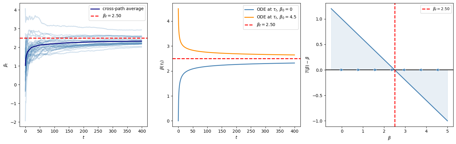
Fig. 101.1 Bray learning dynamics#
REE: β_f = a/(1-b) = 2.5000
Jacobian M = b - 1 = -0.4000  (< 0: E-stable)
The stochastic paths are noisy because prices contain \(\tilde u_t\).
The average path and the ODE paths remove most of that noise and reveal the mean learning direction.
101.8. Counterexample: Unstable Bray feedback#
To see what happens when E-stability is violated, repeat Bray’s model with \(b > 1\).
It represents an economy where expectations affect actual prices more than one-for-one.
If agents start with a forecast that is too high, the market outcome induced by that forecast is higher still, so least squares raises the forecast.
The same logic works in reverse below the REE.
The REE exists, but it is not learnable by this adaptive rule.
The same three diagnostic panels now show how beliefs are pushed away from the REE rather than toward it, and the drift panel shows that the learning force points away from the fixed point on both sides.
b_unstable = 1.4


def T_unstable(β):
    return a_bray + b_unstable * β


β_f_unstable = a_bray / (1 - b_unstable)

β_paths_unstable = simulate_rls_scalar(
    T_unstable, σ_bray, β0=0.0,
    T_periods=200, N_paths=50
)


def ode_unstable(β):
    return T_unstable(β) - β


β_grid = np.linspace(-5, 5, 300)
drift = np.array([ode_unstable(b) for b in β_grid])

t_ode_un, sol_un_low = solve_ode_calendar(ode_unstable, -4.0, 200)
_, sol_un_high = solve_ode_calendar(ode_unstable, 0.0, 200)

fig, axes = plt.subplots(1, 3, figsize=(15, 4.8))

ax = axes[0]
for i in range(min(30, 50)):
    ax.plot(β_paths_unstable[i], color='crimson', alpha=0.3, lw=2)
ax.axhline(β_f_unstable, color='black', ls='--', lw=2,
           label=f'$\\beta_f = {β_f_unstable:.2f}$ (unstable)')
ax.set_xlabel('$t$')
ax.set_ylabel('$\\beta_t$')
ax.legend()

ax = axes[1]
ax.plot(
    t_ode_un, sol_un_low, color='crimson', lw=2,
    label='ODE at $\\tau_t$, $\\beta_0=-4$'
)
ax.plot(
    t_ode_un, sol_un_high, color='steelblue', lw=2,
    label='ODE at $\\tau_t$, $\\beta_0=0$'
)
ax.axhline(β_f_unstable, color='black', ls='--', lw=2,
           label=f'$\\beta_f = {β_f_unstable:.2f}$')
ax.set_xlabel('$t$')
ax.set_ylabel('$\\beta(\\tau_t)$')
ax.legend()

plot_scalar_drift(
    axes[2], β_grid, drift, β_f_unstable, 'crimson'
)

plt.tight_layout()
plt.show()
print(f"Jacobian M = b - 1 = {b_unstable - 1:.2f}  (> 0: NOT E-stable)")
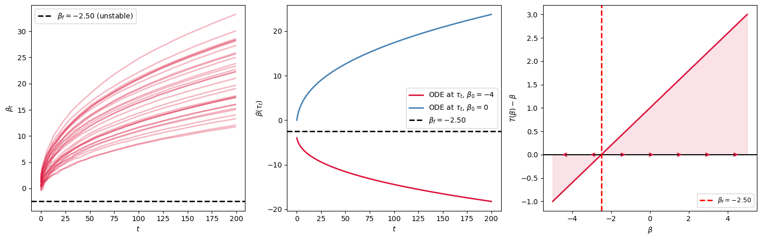
Fig. 101.2 Unstable Bray dynamics#
Jacobian M = b - 1 = 0.40 (> 0: NOT E-stable)
101.9. Example 3: Bray-Savin supply-shifter model#
Bray and Savin [1986] studied a model where
with \(x_t\) an exogenous supply-shifter, \(a\) a scalar feedback parameter, and agents running an OLS regression of \(p\) on \(x\).
This is the same learning problem with one extra economic ingredient: expectations are conditional on an observed shifter.
Agents do not merely forecast the average price.
They estimate how price responds to \(x_t\).
The actual coefficient on \(x_t\) is \(m+a\beta\), so the perceived slope changes the true slope generated by the market.
If \(a < 1\), a mistaken slope feeds back into the actual price equation with attenuation, and the least-squares estimate is pulled toward the REE slope.
The mapping is \(T(\beta) = m + a\beta\) (scalar case), giving
with Jacobian \(\mathcal{M} = a - 1 < 0\) iff \(a < 1\).
The simulation below draws the exogenous shifter \(x_t\) and lets agents update the slope in the regression of \(p_t\) on \(x_t\).
It uses \(a=0.7\).
The drift panel shows that mistaken slopes are pushed back toward the REE slope rather than amplified.
The next cell adapts the RLS simulator to the supply-shifter regression.
def simulate_bray_savin(m, a, σ_x, σ_u, β0, T_periods=500,
                        N_paths=100, seed=0):
    """
    Simulate RLS for p_t = x_t (m + a β_t) + u_t.
    Agents regress p_t on x_t.
    """
    rng = np.random.default_rng(seed)
    β_paths = np.empty((N_paths, T_periods))

    for i in range(N_paths):
        β = β0
        R = 1.0

        for t in range(T_periods):
            x_t = rng.normal(0.0, σ_x)
            u_t = rng.normal(0.0, σ_u)
            p_t = x_t * (m + a * β) + u_t
            step = 1.0 / (t + 1)

            R_old = max(R, 1e-8)
            β = β + step / R_old * x_t * (p_t - β * x_t)
            R = R + step * (x_t**2 - R)
            R = max(R, 1e-8)
            β_paths[i, t] = β

    return β_paths
m_bs, a_bs = 0.5, 0.7
σ_x_bs, σ_u_bs = 1.0, 1.0


def T_bs(β):
    return m_bs + a_bs * β


β_f_bs = m_bs / (1 - a_bs)

β_paths_bs = simulate_bray_savin(
    m_bs, a_bs, σ_x_bs, σ_u_bs, 0.0,
    T_periods=T_sim, N_paths=N_sim
)


def ode_bs(β):
    return T_bs(β) - β


t_ode_bs, sol_bs_low = solve_ode_calendar(ode_bs, 0.0, T_sim)
_, sol_bs_high = solve_ode_calendar(ode_bs, 4.0, T_sim)

β_grid_bs = np.linspace(-0.5, 4.0, 300)
drift_bs = np.array([ode_bs(b) for b in β_grid_bs])

fig, axes = plt.subplots(1, 3, figsize=(15, 4.8))

ax = axes[0]
for i in range(min(30, N_sim)):
    ax.plot(β_paths_bs[i], color='darkorange', alpha=0.25, lw=2)
ax.plot(np.mean(β_paths_bs, axis=0), color='saddlebrown', lw=2,
        label='cross-path average')
ax.axhline(β_f_bs, color='red', ls='--', lw=2,
           label=f'$\\beta_f = {β_f_bs:.2f}$')
ax.set_xlabel('$t$')
ax.set_ylabel('$\\beta_t$')
ax.legend()

ax = axes[1]
ax.plot(
    t_ode_bs, sol_bs_low, color='darkorange', lw=2,
    label='ODE at $\\tau_t$, $\\beta_0=0$'
)
ax.plot(
    t_ode_bs, sol_bs_high, color='steelblue', lw=2,
    label='ODE at $\\tau_t$, $\\beta_0=4$'
)
ax.axhline(β_f_bs, color='red', ls='--', lw=2,
           label=f'$\\beta_f = {β_f_bs:.2f}$')
ax.set_xlabel('$t$')
ax.set_ylabel('$\\beta(\\tau_t)$')
ax.legend()

plot_scalar_drift(
    axes[2], β_grid_bs, drift_bs, β_f_bs, 'darkorange'
)

plt.tight_layout()
plt.show()
print(f"REE: β_f = m/(1-a) = {β_f_bs:.4f}")
print(f"Jacobian M = a - 1 = {a_bs - 1:.4f}  (< 0: E-stable)")
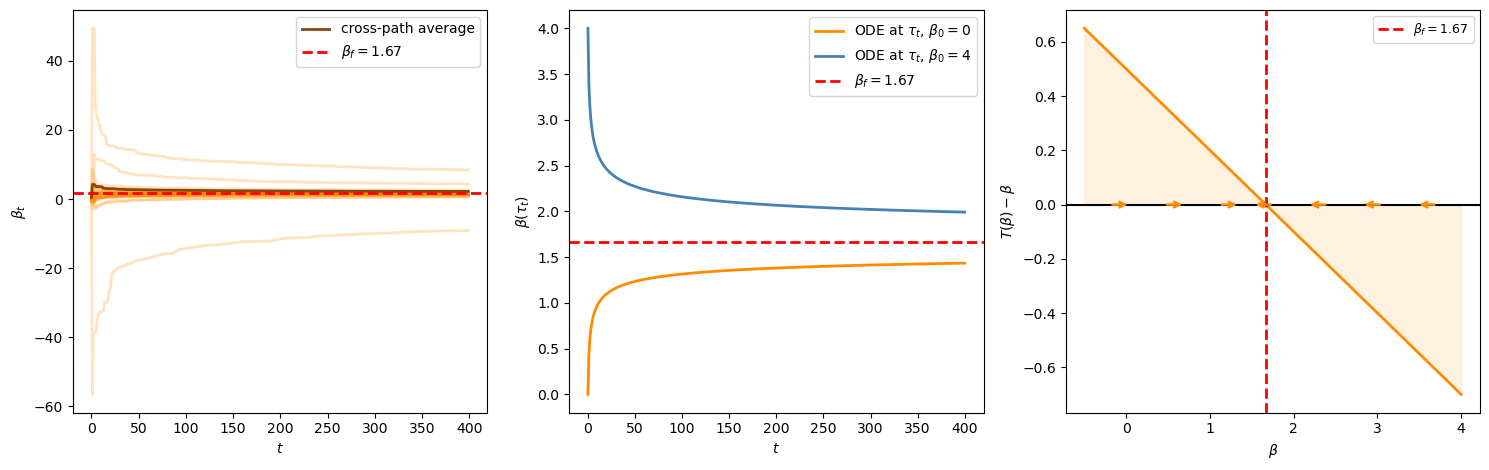
Fig. 101.3 Bray-Savin learning dynamics#
REE: β_f = m/(1-a) = 1.6667
Jacobian M = a - 1 = -0.3000  (< 0: E-stable)
The interpretation is parallel to Bray’s cobweb model.
The difference is that agents are now learning how prices co-move with an exogenous variable, not just learning an unconditional mean.
101.10. Example 4: Hyperinflation / asset prices#
Consider the present-value asset pricing model
where \(|\lambda| < 1\), \(|\rho| < 1\), and agents perceive \(y_t = \beta_t x_{t-1}+ v_t\).
Under the perceived law, \(\mathbb{E}_t y_{t+1} = \beta_t x_t\), so (101.15) becomes
The coefficient on \(x_{t-1}\) in the actual law of motion is therefore \((\lambda \beta_t + 1)\rho\), which gives the operator \(T\) below.
If \(y_t\) is a price level, the equation resembles a Cagan-style hyperinflation model.
If \(y_t\) is an asset price and \(x_t\) is a dividend or fundamental, it is a present-value relation.
In both cases, beliefs about the future value of \(y\) enter the current value of \(y\).
The product \(\lambda\rho\) measures the strength of the forward-looking feedback: \(\lambda\) discounts the future and \(\rho\) measures how persistent the fundamental is.
When \(|\lambda\rho|<1\), a mistaken perceived coefficient does not amplify without bound.
The mapping is \(T(\beta) = (\lambda\beta + 1)\rho\) and the REE is
The small ODE is
with Jacobian \(\mathcal{M} = \lambda\rho - 1 < 0\) for \(|\lambda\rho| < 1\), so the small ODE is stable.
The convergence theorem then applies under the exogenous-regressor conditions above.
The simulation uses \(\lambda=0.8\) and \(\rho=0.9\), so \(\lambda\rho=0.72\).
This means the feedback from expectations is strong enough to matter but still less than one.
The ODE panel below uses \(\tau\) itself on the horizontal axis, where \(\tau\) is the total step size accumulated by least squares.
The code simulates the autoregressive fundamental \(x_t\) and updates an OLS regression of \(y_t\) on \(x_{t-1}\).
The next cell simulates the autoregressive fundamental and the matching RLS update.
It keeps the covariance estimate \(R_t\) bounded away from zero, mirroring the projection idea above and avoiding misleading early-sample explosions.
def simulate_present_value_rls(λ, ρ, σ_ε, β0, T_periods=500,
                               N_paths=100, seed=0):
    """
    Simulate RLS for y_t = (λ β_t + 1) x_t,
    x_t = ρ x_{t-1} + ε_t, with regression of y_t on x_{t-1}.
    """
    rng = np.random.default_rng(seed)
    β_paths = np.empty((N_paths, T_periods))
    σ_x = σ_ε / np.sqrt(1 - ρ**2)
    R_min = 0.05 * σ_x**2

    for i in range(N_paths):
        β = β0
        R = σ_x**2
        x_lag = rng.normal(0.0, σ_x)

        for t in range(T_periods):
            ε_t = rng.normal(0.0, σ_ε)
            x_t = ρ * x_lag + ε_t
            y_t = (λ * β + 1.0) * x_t
            step = 1.0 / (t + 1)

            R_old = max(R, R_min)
            β = β + step / R_old * x_lag * (y_t - β * x_lag)
            R = R + step * (x_lag**2 - R)
            R = max(R, R_min)
            β_paths[i, t] = β
            x_lag = x_t

    return β_paths
λ, ρ_pv, σ_pv = 0.8, 0.9, 1.0
T_pv_sim = T_sim
N_pv_sim = N_sim


def T_pv(β):
    return (λ * β + 1) * ρ_pv


β_f_pv = ρ_pv / (1 - λ * ρ_pv)

β_paths_pv = simulate_present_value_rls(
    λ, ρ_pv, σ_pv, 0.0,
    T_periods=T_pv_sim, N_paths=N_pv_sim
)


def ode_pv(β):
    return T_pv(β) - β


τ_grid_pv = np.linspace(0.0, 30.0, 300)
sol_pv_low = solve_ivp(
    lambda τ, y: [ode_pv(y[0])],
    (0.0, τ_grid_pv[-1]),
    [0.0],
    t_eval=τ_grid_pv,
    max_step=0.05
).y[0]
sol_pv_high = solve_ivp(
    lambda τ, y: [ode_pv(y[0])],
    (0.0, τ_grid_pv[-1]),
    [10.0],
    t_eval=τ_grid_pv,
    max_step=0.05
).y[0]

β_grid_pv = np.linspace(-1.0, 7.0, 300)
drift_pv = np.array([ode_pv(b) for b in β_grid_pv])

fig, axes = plt.subplots(1, 3, figsize=(15, 4.8))

ax = axes[0]
for i in range(min(30, N_pv_sim)):
    ax.plot(β_paths_pv[i], color='seagreen', alpha=0.25, lw=2)
ax.plot(np.mean(β_paths_pv, axis=0), color='darkgreen', lw=2,
        label='cross-path average')
ax.axhline(β_f_pv, color='red', ls='--', lw=2,
           label=f'$\\beta_f = {β_f_pv:.2f}$')
ax.set_xlabel('$t$')
ax.set_ylabel('$\\beta_t$')
ax.legend()

ax = axes[1]
ax.plot(
    τ_grid_pv, sol_pv_low, color='seagreen', lw=2,
    label='ODE, $\\beta_0=0$'
)
ax.plot(
    τ_grid_pv, sol_pv_high, color='steelblue', lw=2,
    label='ODE, $\\beta_0=10$'
)
ax.axhline(β_f_pv, color='red', ls='--', lw=2,
           label=f'$\\beta_f = {β_f_pv:.2f}$')
ax.set_xlabel('Accumulated step size $\\tau$')
ax.set_ylabel('$\\beta(\\tau)$')
ax.legend()

plot_scalar_drift(
    axes[2], β_grid_pv, drift_pv, β_f_pv, 'seagreen'
)

plt.tight_layout()
plt.show()
print(f"REE: β_f = ρ/(1 - lambda*ρ) = {β_f_pv:.4f}")
print(f"Jacobian M = lambda*ρ - 1 = {λ*ρ_pv - 1:.4f}  (< 0: E-stable)")
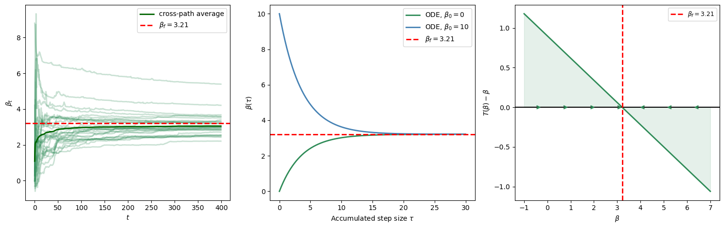
Fig. 101.4 Present-value learning dynamics#
REE: β_f = ρ/(1 - lambda*ρ) = 3.2143
Jacobian M = lambda*ρ - 1 = -0.2800  (< 0: E-stable)
The REE coefficient is larger than \(\rho\) because current prices capitalize expected future fundamentals.
Learning converges because each revision in \(\beta_t\) changes expectations, but the discounted persistence term \(\lambda\rho\) prevents revisions from feeding back explosively.
101.11. Example 5: Investment under uncertainty#
Let’s now consider a version of the Lucas-Prescott investment model where agents learn about the aggregate capital stock \(K_t\) by regressing on \((K_{t-1}, w_{t-1})\) where \(w_t\) is an exogenous cost shock.
Firms choose investment using a perceived law of motion for aggregate capital.
Those investment choices then determine the actual law of motion for aggregate capital through market clearing.
Learning is therefore about a state variable that agents themselves help create through their investment decisions.
The perceived law of motion is
while the actual law (from firms’ optimal investment decisions and market clearing) is
where the nonlinear mappings \(T_1, T_2\) come from solving the firms’ linear quadratic control problems.
The two coefficients have different economic roles.
\(\beta_1\) describes persistence in aggregate capital, while \(\beta_2\) describes how the exogenous shock \(w_t\) affects next period’s capital.
Because the optimal investment rule depends on the whole perceived law of motion, the map \(T\) is nonlinear.
This is why the larger ODE is harder to analyze here than in the scalar examples with exogenous regressors.
The small ODE decomposes as:
and E-stability can be verified analytically for \(|\beta_1| < b^{-1/2}\) (where \(b\) is the discount factor).
The phase portrait below plots the vector field \(T(\beta)-\beta\) over \((\beta_1,\beta_2)\) space.
Each arrow shows how the perceived law of motion would be revised if the economy were currently operating under that belief.
The plotted trajectories are deterministic ODE paths, not noisy least-squares sample paths.
def T_invest(β, b=0.95, d=1.0, f=1.0, A1=1.0, N=1.0, ρ_w=0.5):
    """Mapping T for the investment model with β = [β1, β2]."""
    b1, b2 = β
    denom1 = 1 - b1 * b + (1 / d) * f**2 * A1 * N
    T1 = (1 - b1 * b) / denom1
    numer2 = 1 - b1 * b + f**2 * A1 * b2 * b * ρ_w
    T2 = (-N / (d * (1 - ρ_w * b))) * (numer2 / denom1) * ρ_w
    return np.array([T1, T2])


def ode_invest(t, β, **kwargs):
    Tb = T_invest(β, **kwargs)
    return Tb - β


params = dict(b=0.95, d=1.0, f=1.0, A1=1.0, N=1.0, ρ_w=0.5)
β1_bound = params["b"] ** (-0.5)
β_f_inv = fsolve(lambda b: T_invest(b, **params) - b, [0.5, 0.1])
print(f"REE: β_f = {β_f_inv}")

eps = 1e-6
J = np.zeros((2, 2))
for j in range(2):
    e = np.zeros(2)
    e[j] = eps
    J[:, j] = (
        T_invest(β_f_inv + e, **params)
        - T_invest(β_f_inv - e, **params)
    ) / (2 * eps)
M = J - np.eye(2)
eigs = la.eigvals(M)
print(f"Jacobian M eigenvalues: {eigs}")
print(f"E-stable: {np.all(eigs.real < 0)}")

fig, ax = plt.subplots(figsize=(8, 6))

b1_grid = np.linspace(-0.1, min(1.0, β1_bound - 1e-3), 20)
b2_grid = np.linspace(-0.8, 0.5, 20)
B1, B2 = np.meshgrid(b1_grid, b2_grid)
U = np.zeros_like(B1)
V_field = np.zeros_like(B2)
for i in range(B1.shape[0]):
    for j in range(B1.shape[1]):
        β_ij = np.array([B1[i, j], B2[i, j]])
        drift = T_invest(β_ij, **params) - β_ij
        U[i, j] = drift[0]
        V_field[i, j] = drift[1]

speed = np.sqrt(U**2 + V_field**2)
speed[speed == 0] = 1e-8
ax.streamplot(b1_grid, b2_grid, U, V_field, color=speed,
              cmap='Blues', density=1.3, linewidth=1)

starts = [(0.1, 0.0), (0.9, 0.4), (0.98, -0.6), (0.3, -0.7)]
colors_traj = ['red', 'darkorange', 'green', 'purple']
for (b10, b20), col in zip(starts, colors_traj):
    sol = solve_ivp(lambda t, β: ode_invest(t, β, **params),
                    [0, 30], [b10, b20],
                    t_eval=np.linspace(0, 30, 300),
                    method='RK45')
    ax.plot(sol.y[0], sol.y[1], color=col, lw=2)
    ax.plot(b10, b20, 'o', color=col, ms=7)

ax.plot(*β_f_inv, 'k*', ms=14, label='REE $\\beta_f$')
ax.set_xlabel('$\\beta_1$', fontsize=12)
ax.set_ylabel('$\\beta_2$', fontsize=12)
ax.legend()
plt.tight_layout()
plt.show()
REE: β_f = [ 0.38728475 -0.28879438]
Jacobian M eigenvalues: [-1.27718071 -1.35664898]
E-stable: True
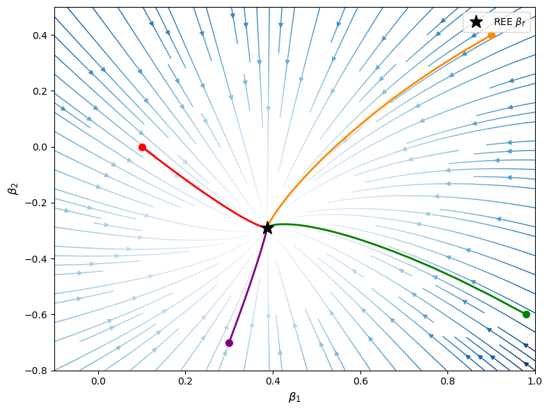
Fig. 101.5 Investment phase portrait#
The star marks the REE.
The paths converge because the capital-persistence coefficient \(\beta_1\) is stabilized first, and then the shock coefficient \(\beta_2\) adjusts given the limiting value of \(\beta_1\).
This recursive structure is why the small ODE is tractable even though the full least-squares system has endogenous regressors.
101.12. Connection to rational learning#
The framework of Marcet and Sargent [1989] belongs to the program of learning about a rational expectations equilibrium, as distinct from learning within one — a distinction emphasized by Bray and Kreps [1987].
Learning within an REE (the subject of the companion lecture Rational Learning and Rational Expectations) refers to Bayesian inference inside a correctly specified model.
In that setting the data-generating process is stationary from the agent’s perspective, and Bayes’ rule is fully rationalized.
Learning about an REE involves an agent who does not know the equilibrium price function.
Because the agent’s beliefs shift the equilibrium price, the data the agent uses to update beliefs are themselves generated by a non-stationary process.
As Marcet and Sargent [1989] put it,
The models do not incorporate fully optimal behavior or rational expectations, because agents operate under the continually falsified assumption that the law of motion is time invariant and known for sure.
Yet it is a compelling rule.
Convergence holds despite the misspecification whenever E-stability combines with the required boundedness and domain-of-attraction conditions.
Unlike Bayesian learning, it does not require strong prior assumptions about the statistical structure of the economy.
101.13. Summary#
This lecture studied least-squares learning in the self-referential models of Marcet and Sargent [1989].
The central object is the map \(T\) from a perceived law of motion to the actual law of motion generated when agents act on that perception.
A rational expectations equilibrium is a fixed point of this map.
Recursive least squares converges to that fixed point when the associated ODE \(\dot\beta = T(\beta)-\beta\) is locally stable and the learning process remains in a region where the model is well defined.
It complements rational learning, studied in Rational Learning and Rational Expectations, where Bayesian agents learn within an equilibrium structure that is already specified.
101.14. Exercises#
Exercise 101.1
Consider the scalar model with \(T(\beta) = a + b\beta\).
Derive a formula for the unique REE \(\beta_f\) in terms of \(a\) and \(b\).
Show that the small ODE \(\dot\beta = T(\beta) - \beta\) is globally stable if and only if \(b < 1\).
Simulate \(N = 200\) paths of length \(T = 500\) for \(a = 1\) and each of \(b \in \{0.3, 0.7, 0.9, 0.99\}\) (all less than 1).
Plot the cross-path average of \(\beta_t\) for each \(b\) value on the same figure and comment on how the rate of convergence changes as \(b \to 1\).
Solution
Here is one solution:
Part 1. The REE satisfies \(\beta_f = T(\beta_f) = a + b\beta_f\), so
Part 2. The small ODE is \(\dot\beta = a + b\beta - \beta = a - (1-b)\beta\).
This is linear with slope \(-(1-b)\), so the unique fixed point \(\beta_f = a/(1-b)\) is globally stable iff \(1-b > 0\), i.e., \(b < 1\).
Part 3.
a_ex, T_ex, N_ex = 1.0, 500, 200
b_values = [0.3, 0.7, 0.9, 0.99]
colors_ex = ['steelblue', 'darkorange', 'seagreen', 'purple']

fig, ax = plt.subplots(figsize=(11, 5))
for b_val, col in zip(b_values, colors_ex):
    def T_fn(β, b_val=b_val):
        return a_ex + b_val * β

    paths = simulate_rls_scalar(T_fn, σ_u=1.0, β0=0.0,
                                T_periods=T_ex, N_paths=N_ex, seed=0)
    bf = a_ex / (1 - b_val)
    ax.plot(np.mean(paths, axis=0), color=col, lw=2,
            label=f'$b={b_val}$, $\\beta_f={bf:.2f}$')

ax.set_xlabel('$t$')
ax.set_ylabel('$E[\\beta_t]$')
ax.set_title('Convergence Rate Slows as $b \\to 1$')
ax.legend()
plt.tight_layout()
plt.show()
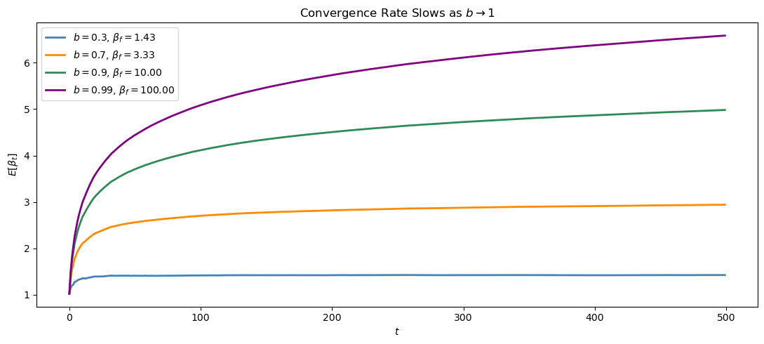
As \(b \to 1\), the Jacobian \(\mathcal M = b - 1\) approaches zero, so the ODE becomes slow to return to the fixed point.
Convergence still occurs, but it takes longer.
Exercise 101.2
Proposition 101.3 states that \(\mathbb{P}(\beta_t \to \hat\beta) = 0\) for any \(\hat\beta \neq \beta_f\) in the interior.
Using the Bray model with \(a=1\), \(b=0.6\), simulate 100 paths of length \(T = 600\) starting from \(\beta_0 = 6\) (far from \(\beta_f = 2.5\)) and show that paths still converge to \(\beta_f\).
Now consider the unstable case \(b = 1.5\), simulate 50 paths of length \(T = 200\) starting from \(\beta_0 = -1.9\) (close to the REE \(\beta_f = -2\)), and describe what happens.
Solution
Here is one solution:
Parts 1 and 2.
fig, axes = plt.subplots(1, 2, figsize=(14, 5))

def T_st(β):
    return 1.0 + 0.6 * β


paths_far = simulate_rls_scalar(T_st, 1.0, β0=6.0,
                                T_periods=600, N_paths=100, seed=1)
ax = axes[0]
for i in range(40):
    ax.plot(paths_far[i], color='steelblue', alpha=0.2, lw=2)
ax.plot(np.mean(paths_far, axis=0), color='navy', lw=2, label='average')
ax.axhline(2.5, color='red', ls='--', lw=2, label='$\\beta_f = 2.5$')
ax.set_title('Stable ($b=0.6$): far start still converges')
ax.set_xlabel('$t$')
ax.set_ylabel('$\\beta_t$')
ax.legend()

def T_un(β):
    return 1.0 + 1.5 * β


β_f_un = 1.0 / (1 - 1.5)
paths_un = simulate_rls_scalar(T_un, 1.0, β0=-1.9,
                               T_periods=200, N_paths=50, seed=2)
ax = axes[1]
for i in range(50):
    ax.plot(paths_un[i], color='crimson', alpha=0.3, lw=2)
ax.axhline(β_f_un, color='black', ls='--', lw=2,
           label=f'$\\beta_f = {β_f_un}$ (unstable)')
ax.set_title('Unstable ($b=1.5$): diverges even near REE')
ax.set_xlabel('$t$')
ax.set_ylabel('$\\beta_t$')
ax.legend()

plt.tight_layout()
plt.show()
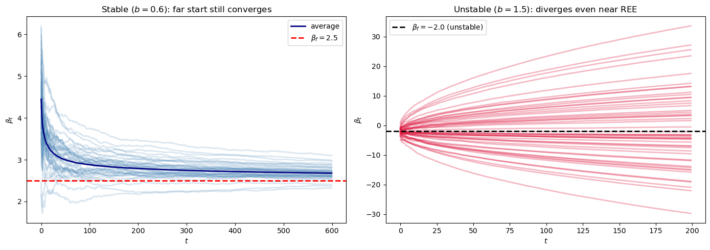
Geometrically, the slope \(dT/d\beta - 1 = b - 1 = 0.5\) is positive at the REE.
The ODE therefore pushes \(\beta\) away from \(\beta_f\) in both directions.
Exercise 101.3
The present-value model: effect of \(\lambda\) on E-stability
In the present-value model (101.15), \(T(\beta) = (\lambda\beta + 1)\rho\) and the Jacobian is \(\mathcal{M} = \lambda\rho - 1\).
For \(\rho = 0.9\) and each of \(\lambda \in \{0.5, 0.8, 0.95, 0.99\}\), compute \(\beta_f\) and \(\mathcal{M}\) and determine whether the REE is E-stable.
For the E-stable cases, simulate 100 paths of length \(T=400\) and plot representative noisy paths in calendar time, then plot the limiting ODE paths in accumulated-gain time.
At \(\lambda = 0.99\), \(\mathcal{M} = 0.99\rho - 1 < 0\).
Simulate paths for this near-boundary case and compare the convergence speed with the \(\lambda = 0.5\) case, providing an intuitive explanation.
Solution
Here is one solution:
Part 1.
ρ_ex = 0.9
λ_values = [0.5, 0.8, 0.95, 0.99]

print(f"{'lambda':>8}  {'β_f':>10}  {'M = λ*ρ-1':>15}  {'E-stable':>10}")
print("-" * 50)
for lv in λ_values:
    bf = ρ_ex / (1 - lv * ρ_ex) if abs(lv * ρ_ex) < 1 else float('inf')
    M_jac = lv * ρ_ex - 1
    estab = "YES" if M_jac < 0 else "NO"
    print(f"{lv:>8.2f}  {bf:>10.4f}  {M_jac:>15.4f}  {estab:>10}")
  lambda         β_f        M = λ*ρ-1    E-stable
--------------------------------------------------
    0.50      1.6364          -0.5500         YES
    0.80      3.2143          -0.2800         YES
    0.95      6.2069          -0.1450         YES
    0.99      8.2569          -0.1090         YES
Parts 2 and 3.
fig, axes = plt.subplots(len(λ_values), 2, figsize=(13, 14))
colors_λ = ['steelblue', 'darkorange', 'seagreen', 'purple']

for row, (lv, col) in enumerate(zip(λ_values, colors_λ)):
    def ode_fn(β, λ_val=lv):
        return (λ_val * β + 1) * ρ_ex - β

    bf = ρ_ex / (1 - lv * ρ_ex)

    paths_λ = simulate_present_value_rls(
        lv, ρ_ex, 1.0, β0=0.0,
        T_periods=400, N_paths=100, seed=3
    )

    ax = axes[row, 0]
    for i in range(20):
        ax.plot(paths_λ[i], color=col, alpha=0.2, lw=2)
    ax.axhline(bf, color='red', ls=':', lw=2,
               label=f'$\\beta_f={bf:.2f}$')
    ax.set_title(f'RLS paths, $\\lambda={lv}$')
    ax.set_xlabel('$t$')
    ax.set_ylabel('$\\beta_t$')
    ax.legend(fontsize=8)

    τ_grid = np.linspace(0.0, 30.0, 300)
    sol_low = solve_ivp(
        lambda τ, y: [ode_fn(y[0])],
        (0.0, τ_grid[-1]),
        [0.0],
        t_eval=τ_grid,
        max_step=0.05
    ).y[0]
    sol_high = solve_ivp(
        lambda τ, y: [ode_fn(y[0])],
        (0.0, τ_grid[-1]),
        [1.5 * bf],
        t_eval=τ_grid,
        max_step=0.05
    ).y[0]

    ax = axes[row, 1]
    ax.plot(τ_grid, sol_low, color=col, lw=2,
            label='ODE, $\\beta_0=0$')
    ax.plot(τ_grid, sol_high, color='black', ls='--', lw=2,
            label='ODE, high start')
    ax.axhline(bf, color='red', ls=':', lw=2,
               label=f'$\\beta_f={bf:.2f}$')
    M_jac = lv * ρ_ex - 1
    ax.set_title(f'ODE, $\\mathcal{{M}}={M_jac:.3f}$')
    ax.set_xlabel('Accumulated step size $\\tau$')
    ax.set_ylabel('$\\beta(\\tau)$')
    ax.legend(fontsize=8)

plt.tight_layout()
plt.show()
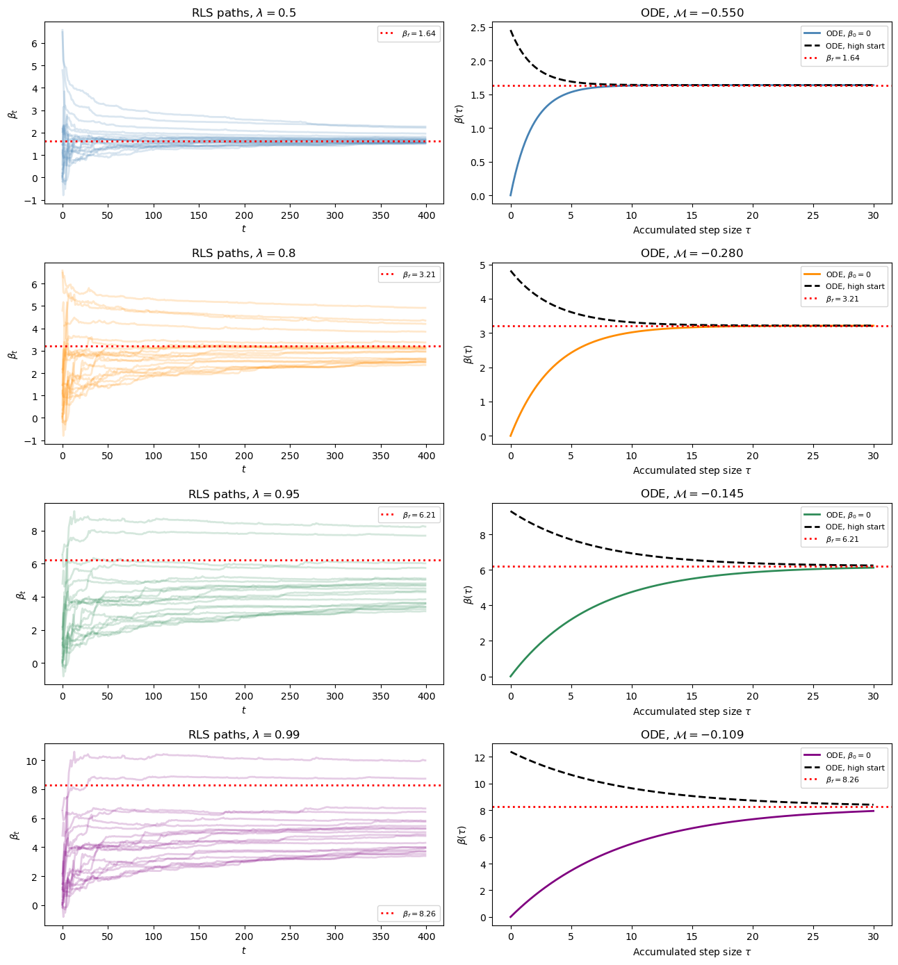
In each row, the left panel shows finite-sample RLS paths in calendar time and the right panel shows deterministic ODE paths in accumulated-gain time.
When \(\lambda=0.99\), \(\mathcal M = 0.99\rho-1 \approx -0.109\) is small in absolute value.
The ODE is nearly flat near \(\beta_f\), so the restoring force is weak and convergence is slow.
When \(\lambda=0.5\), \(\mathcal M=-0.55\), which gives a stronger restoring force and faster convergence.