100. Rational Learning and Rational Expectations#
100.1. Overview#
This lecture explores an important question in economic theory: what can agents learn inside a rational expectations equilibrium?
This question is related to, but distinct from, the adaptive-learning question of whether a rational expectations equilibrium can be justified as a dynamic attractor.
The starting point is Bray and Kreps [1987], which gives a rigorous model of Bayesian learning inside a rational expectations equilibrium.
In a rational expectations equilibrium, agents use market prices to make inferences about other agents’ private information.
Each agent knows the statistical relationship between prices and the underlying payoff-relevant variables and that relationship is correct given the equilibrium.
But this raises a question: where does that knowledge come from?
Their rational learning approach answers a narrower question.
Agents are uncertain about structural parameters, and the state space is enlarged to include, for each candidate value, the associated equilibrium price and allocation maps.
Agents then use Bayes’ rule to update over those possibilities as prices and returns are observed.
This lecture develops that Bayesian formulation through an asset-market model.
The aim is to see what rational learning can explain, and where its limits appear, before turning to the computational illustration.
The discussion also connects to earlier work by Bray [1982], Bray and Savin [1986], and the rational expectations literature of Radner [1979], Grossman [1976], and Jordan [1982].
Let’s start with the following imports
import numpy as np
import matplotlib.pyplot as plt
from scipy.optimize import brentq
100.2. The economy#
The model is a simple asset market built around the recurring information model of Grossman and Stiglitz [1980], repeated across infinitely many dates.
100.2.1. Agents and assets#
Each date is economically disconnected from the others, so agents start each period afresh.
There are two types of agents and two assets:
A safe asset with net return normalized to zero.
A risky asset endowed one unit per agent and traded at date \(t\) at spot price \(p_t\).
At each date \(t = 0, 1, 2, \ldots\) the risky asset yields a gross return \(r_t\) at date \(t+1/2\).
An informed signal \(s_t\) satisfies
where \(\{s_t\}\) and \(\{\epsilon_t\}\) are IID normal sequences and are mutually independent.
Common knowledge of the prior moments \((\mu_s, \tau^2)\) is what makes the price observation informative about \(\theta^I\), as we will see.
There are two representative agents:
Agent \(I\) (informed) observes \(s_t\) before trading at date \(t\).
Agent \(U\) (uninformed) observes the equilibrium price \(p_t\) but not \(s_t\) before trading.
Both agents observe the previous return before current trading.
100.2.2. Preferences#
Agent \(n \in \{I, U\}\) has constant absolute risk tolerance \(\theta^n\).
If agent \(n\) holds \(x^n\) units of the risky asset and \(y^n\) units of the safe asset between dates \(t\) and \(t+1/2\), period utility is
Thus \(1/\theta^n\) is the coefficient of absolute risk aversion.
Given the signal \(s_t\), the informed agent’s demand is
Because each of the two agents is endowed with one unit of the risky asset, market clearing is
100.2.3. Rational expectations equilibrium#
If all agents knew \(s_t\), agent \(n\) would demand
With \(N\) agents and total risky-asset supply \(N\), market clearing gives the full communication equilibrium price
Thus if \(\sum_n \theta^n\) is known, the price fully reveals \(s_t\).
Following Radner [1979], this is called a full communication rational expectations equilibrium.
Suppose now that \(\theta^I\) is unknown to agent \(U\).
Following Bray and Kreps [1987], we treat this uncertainty by expanding the state space: we let the unknown parameter \(\theta^I\) become a coordinate of the state, alongside the per-period shocks \((s_t, \epsilon_t)\).
Formally, the state space is \(\Omega = \Theta \times \Phi^\infty\), where \(\Theta = [a,b]\) supports the unknown \(\theta^I\) and \(\Phi\) supports each \((s_t, \epsilon_t)\).
Agent \(U\) knows \(\sigma^2\) and \(\theta^U\), and starts with a prior density over \(\theta^I\) on \([a,b]\).
This expansion is what turns the learning problem into Bayesian inference inside a single rational expectations equilibrium on \(\Omega\).
At a date when agent \(U\) has posterior density \(f\) over \(\theta^I\), his own trade reveals \(x^I_t=2-x^U_t\) through market clearing.
Combining this inferred \(x^I_t\) with (100.1), each candidate \(\theta^I\) implies
After trading, agent \(U\) observes \(r_t\).
Bayes’ rule then updates the posterior over \(\theta^I\) using the normal density of the signal implied by (100.3) conditional on the realized return.
This is the main object learned in the two-agent example.
Even in this simple case, the equilibrium can be defined recursively but closed-form prices are unavailable.
100.3. The rational learning equilibrium#
The model has two pieces that interact at each date.
The first is the within-period equilibrium given the uninformed agent’s current posterior on \(\theta^I\).
The second is the Bayesian update of that posterior after the period closes.
100.3.1. Uninformed demand given beliefs#
Suppose at date \(t\) agent \(U\) has posterior density \(f_t\) on \(\theta^I\), supported on \([a, b]\).
Suppose the equilibrium price is \(p\) and the equilibrium informed trade \(X^I = 2 - x^U\) has been inferred from market clearing.
Conditional on \(\theta\), equation (100.3) pins down the signal as \(s_t(\theta) = \sigma^2 X^I/\theta + p\).
Two sources of information about \(\theta\) are therefore present at the start of date \(t\) trading: the carried-over posterior \(f_t(\theta)\) and the Gaussian prior \(\phi_s(\cdot;\mu_s,\tau^2)\) on \(s_t\) that values some implied signals as more plausible than others.
Bayes’ rule combines them into the intra-period posterior
which is the posterior on \(\theta^I\) that the agent actually uses to forecast \(r_t\) before \(r_t\) is observed.
Conditional on a candidate value \(\theta\), the excess payoff on one unit of the risky asset is
Because CARA preferences have no wealth effects, agent \(U\)’s problem reduces to
where the expectation integrates over \(\theta^I \sim f_t^{(p, X^I)}\) and \(\epsilon_t\).
Substituting the conditional excess payoff and using the normal moment-generating formula gives
up to a \(\theta\)-independent constant absorbed in normalisation.
Define the tilted weight
The first-order condition rearranges to
The right-hand side is \(X^I\) multiplied by a tilted expectation of \(1/\theta^I\) under the weighting in (100.5).
Equation (100.6) implicitly defines \(x^U(p, X^I; f_t)\), the uninformed agent’s optimal demand at observed price \(p\), conjectured informed trade \(X^I\), and prior posterior \(f_t\).
Dependence on \(p\) enters through the prior weight \(\phi_s\): at higher prices, candidate values of \(\theta\) that imply \(s_t\) above the prior mean become less plausible, so the agent’s demand schedule slopes downward in \(p\) as expected.
100.3.2. Market clearing#
Equilibrium requires that the informed and uninformed demands sum to the total endowment.
Substituting (100.1) and the implicit function \(x^U(p, X^I; f_t)\), the equilibrium \((p_t, X^I_t)\) satisfies the two equations
Eliminating \(X^I_t\) between the two leaves a single root-finding problem for \(p_t\).
Combining the two equations, the equilibrium price has the form
When \(f_t\) collapses to a point mass at the true \(\theta^I\), equation (100.6) simplifies to \(x^U/\theta^U = X^I/\theta^I\), and market clearing gives the full-communication allocation
This is the full-communication allocation we will use to check the simulation.
100.3.3. Bayesian update#
After trading, agent \(U\) observes \((p_t, x^U_t, r_t)\).
Market clearing gives \(X^I_t = 2 - x^U_t\), and equation (100.3) assigns a candidate \(s_t(\theta) = \sigma^2 X^I_t/\theta + p_t\) to each \(\theta\).
Since \(s_t \sim N(\mu_s, \tau^2)\) independently of \(\epsilon_t \sim N(0,\sigma^2)\), the conditional density of \(s_t\) given \(r_t\) is Gaussian:
where \(\phi(\cdot; m, v)\) denotes the Normal density with mean \(m\) and variance \(v\).
Bayes’ rule then produces the posterior update
This is the rule we simulate below.
100.4. Computing the equilibrium#
We discretise the support \([a,b]\) of \(\theta^I\) on a fine grid and represent \(f_t\) as a vector of density values.
The three computational primitives are:
uninformed_demandsolves the FOC in (100.6) for \(x^U(p, X^I; f)\) by root-finding.equilibrium_pricesolves the market-clearing system (100.7) for \(p_t\).bayes_updateapplies (100.10) and renormalises.
def uninformed_demand(p, XI, f, θ_grid, θ_U, σ2, μ_s, τ2):
    """
    Solve the FOC for x^U(p, X^I; f), the uninformed
    agent's optimal demand given observed price p, conjectured
    informed trade XI, and carried-over posterior density f.
    """
    with np.errstate(divide='ignore'):
        log_f = np.log(f)
    s_implied = σ2 * XI / θ_grid + p
    log_phi_s = -0.5 * (s_implied - μ_s)**2 / τ2  # prior weight on s_t

    def foc(xU):
        z = xU * σ2 * XI / (θ_grid * θ_U)
        log_w = log_f + log_phi_s - z
        M = log_w.max()
        w = np.exp(log_w - M)
        num = np.sum(w / θ_grid)
        den = np.sum(w)
        return xU / θ_U - XI * num / den

    return brentq(foc, -50.0, 50.0, xtol=1e-10)
def equilibrium_price(s_t, θ_I_true, f, θ_grid, θ_U, σ2, μ_s, τ2):
    """
    Solve the market-clearing system for the equilibrium
    price p_t given signal s_t, true informed risk tolerance
    θ_I_true, and posterior f.
    """
    def mc_residual(p):
        XI = θ_I_true * (s_t - p) / σ2
        xU = uninformed_demand(p, XI, f, θ_grid, θ_U, σ2, μ_s, τ2)
        return XI + xU - 2.0

    return brentq(mc_residual, s_t - 10.0, s_t, xtol=1e-8)
def bayes_update(f, θ_grid, p_t, xU_t, r_t, σ2, τ2, μ_s):
    """
    Bayesian update of the posterior on θ^I given the date-t
    observations (p_t, x^U_t, r_t).
    """
    XI = 2.0 - xU_t
    s_mean = (σ2 * μ_s + τ2 * r_t) / (σ2 + τ2)
    s_var = σ2 * τ2 / (σ2 + τ2)
    s_implied = σ2 * XI / θ_grid + p_t

    log_like = -0.5 * (s_implied - s_mean)**2 / s_var
    log_like -= log_like.max()  # log-shift for stability
    f_new = f * np.exp(log_like)
    dθ = θ_grid[1] - θ_grid[0]
    f_new /= np.sum(f_new) * dθ
    return f_new
The simulation loop chains \((s_t, \epsilon_t)\) shocks through these three functions.
def simulate(θ_I_true, θ_U, σ2, μ_s, τ2,
             a, b, n_grid, T, prior=None, seed=42):
    """
    Simulate T periods of the Bray-Kreps rational-learning equilibrium.
    """
    rng = np.random.default_rng(seed)
    θ_grid = np.linspace(a, b, n_grid)
    dθ = θ_grid[1] - θ_grid[0]

    if prior is None:
        f = np.ones(n_grid) / (b - a)
    else:
        f = prior(θ_grid)
        f /= np.sum(f) * dθ

    s_seq = rng.normal(μ_s, np.sqrt(τ2), T)
    eps_seq = rng.normal(0.0, np.sqrt(σ2), T)

    XI_path = np.empty(T)
    p_path = np.empty(T)
    r_path = np.empty(T)
    post_mean = np.empty(T + 1)
    post_var = np.empty(T + 1)
    post_mean[0] = np.sum(θ_grid * f) * dθ
    post_var[0] = np.sum((θ_grid - post_mean[0])**2 * f) * dθ

    snap_times = {0, 5, 20, 50, 100, T}
    snapshots = {0: f.copy()}

    for t in range(T):
        p_t = equilibrium_price(
            s_seq[t], θ_I_true, f, θ_grid, θ_U, σ2, μ_s, τ2
        )
        XI = θ_I_true * (s_seq[t] - p_t) / σ2
        xU = 2.0 - XI
        r_t = s_seq[t] + eps_seq[t]
        f = bayes_update(f, θ_grid, p_t, xU, r_t, σ2, τ2, μ_s)

        XI_path[t] = XI
        p_path[t] = p_t
        r_path[t] = r_t
        post_mean[t + 1] = np.sum(θ_grid * f) * dθ
        post_var[t + 1] = np.sum(
            (θ_grid - post_mean[t + 1])**2 * f
        ) * dθ
        if (t + 1) in snap_times:
            snapshots[t + 1] = f.copy()

    return dict(
        θ_grid=θ_grid,
        snapshots=snapshots,
        XI_path=XI_path,
        p_path=p_path,
        r_path=r_path,
        post_mean=post_mean,
        post_var=post_var,
    )
100.5. Posterior concentration#
We run the simulation with a uniform prior on \([0.5, 4]\) and true \(\theta^I = 2\).
params = dict(
    θ_I_true=2.0,
    θ_U=1.0,
    σ2=1.0,
    μ_s=1.0,
    τ2=1.0,
    a=0.5,
    b=4.0,
    n_grid=300,
    T=200,
    seed=42,
)

res = simulate(**params)
The first picture shows snapshots of the posterior density at selected dates.
fig, ax = plt.subplots(figsize=(10, 5))
for t, ft in sorted(res['snapshots'].items()):
    ax.plot(res['θ_grid'], ft, lw=2, label=f't = {t}')
ax.axvline(params['θ_I_true'], color='black', ls='--', lw=1.5,
           label=r'$\theta^I_{\rm true}$')
ax.set_xlabel(r'$\theta^I$')
ax.set_ylabel('posterior density')
ax.legend()
plt.tight_layout()
plt.show()
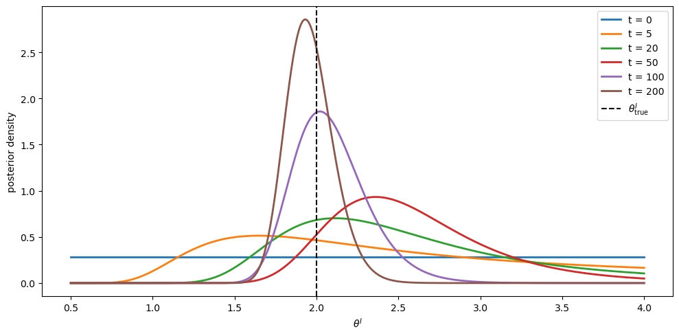
Fig. 100.1 posterior density over \(\theta^I\) at selected dates#
The posterior tightens around \(\theta^I_{\rm true} = 2\) as price and return data accumulate.
The next picture tracks the posterior mean and variance.
fig, axes = plt.subplots(1, 2, figsize=(13, 5))

ax = axes[0]
ax.plot(np.arange(params['T'] + 1), res['post_mean'], lw=2)
ax.axhline(params['θ_I_true'], color='red', ls='--', lw=2,
           label=r'$\theta^I_{\rm true}$')
ax.set_xlabel('$t$')
ax.set_ylabel(r'$E_t[\theta^I]$')
ax.legend()

ax = axes[1]
ax.plot(np.arange(params['T'] + 1), res['post_var'], lw=2)
ax.set_xlabel('$t$')
ax.set_ylabel(r'${\rm Var}_t[\theta^I]$')

plt.tight_layout()
plt.show()
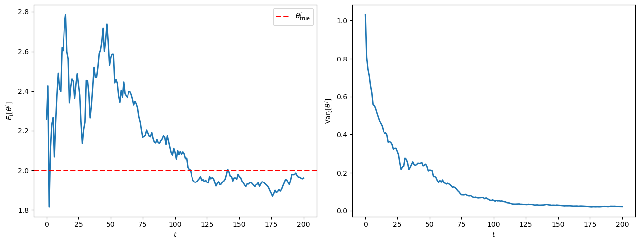
Fig. 100.2 posterior mean and variance over time#
The posterior mean converges to the truth and the posterior variance vanishes.
This is the concrete manifestation of weak convergence of posteriors to a point mass at \(\theta^I_{\rm true}\), which we describe in general terms below.
100.6. Equilibrium trades and prices#
The equilibrium informed trade \(X^I_t\) depends on the current signal \(s_t\), on \(\theta^I_{\rm true}\), and on the carried-over posterior \(f_t\), all through the market-clearing system (100.7).
As \(f_t\) tightens around \(\theta^I_{\rm true}\), the average \(X^I_t\) approaches the full-communication allocation in (100.9).
XI_full = 2 * params['θ_I_true'] / (params['θ_I_true'] + params['θ_U'])
p_mean_full = params['μ_s'] - params['σ2'] * XI_full / params['θ_I_true']

fig, axes = plt.subplots(1, 2, figsize=(13, 5))

ax = axes[0]
ax.plot(res['XI_path'], lw=2, label='$X^I_t$ (learning)')
ax.axhline(XI_full, color='red', ls='--', lw=2,
           label='$X^I$ (full info)')
ax.set_xlabel('$t$')
ax.set_ylabel('$X^I_t$')
ax.legend()

ax = axes[1]
ax.plot(res['p_path'], lw=1.5, alpha=0.7, label='$p_t$ (learning)')
ax.axhline(p_mean_full, color='red', ls='--', lw=2,
           label='$E[p_t]$ (full info)')
ax.set_xlabel('$t$')
ax.set_ylabel('$p_t$')
ax.legend()

plt.tight_layout()
plt.show()
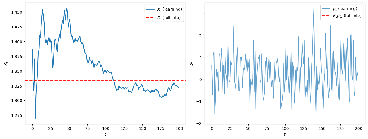
Fig. 100.3 equilibrium trade and prices over time#
The left panel shows \(X^I_t\) approaching the full-information allocation as beliefs concentrate.
The right panel shows the price path, which fluctuates because \(p_t\) inherits the variation in \(s_t\).
The simulation illustrates three features of this equilibrium.
The posterior density on \(\theta^I\) concentrates around the true value, the posterior variance vanishes, and the equilibrium informed trade \(X^I_t\) converges to its full-information benchmark.
The next sections identify the theorems behind these outcomes and the assumptions they require.
We first state the two convergence results of Bray and Kreps [1987] for the abstract model, then specialize to the two-agent example to pin down the hypotheses that drive concentration on the true \(\theta^I\), and finally explain when those hypotheses can fail.
100.7. Convergence of posterior assessments#
Let \((\Omega, \mathcal F)\) be a measurable space carrying the equilibrium.
In the two-agent example, \(\Omega = \Theta \times \Phi^{\infty}\), where \(\Theta = [a,b] \times \{\theta^U\}\) collects the structural parameters, \(\Phi\) collects the per-period shocks \((s_t, \epsilon_t)\), and \(\mathcal F\) is the product Borel \(\sigma\)-field.
Agent \(n\) enters date \(0\) with a prior probability measure \(P^n\) on \((\Omega, \mathcal F)\).
Let \(G_t^n \subseteq \mathcal F\) denote the \(\sigma\)-field generated by agent \(n\)’s private information through date \(t\), and let
be the \(\sigma\)-field that adds observation of equilibrium prices through date \(t\).
The tail \(\sigma\)-field is
The first result, due to Bray and Kreps [1987], states that the conditional probability of any event converges almost surely.
Proposition 100.1
Fix an agent \(n\) and an event \(A \in \mathcal F\).
The process \(M_t = \mathbb{E}^n[\mathbf 1_A \mid H_t^n(p)]\) is a \(P^n\)-bounded martingale with respect to \((H_t^n(p))_{t \ge 0}\), and
The proof is the bounded martingale convergence theorem, with \(M_t \in [0,1]\) supplying the uniform integrability needed for the limit identification.
Proposition 100.1 is convergence of posterior assessments, not convergence to “correct” beliefs.
Two qualifications are worth stating.
The “a.s.” statement is relative to agent \(n\)’s own prior \(P^n\), so if two priors \(P^n\) and \(P^{n'}\) are mutually singular, the conclusion need not hold simultaneously on a common \(P\)-positive event.
If the priors share a common null collection, simultaneous convergence holds outside a common null set.
The second result in Bray and Kreps [1987] sharpens convergence from individual events to the entire posterior measure on the parameter space, given a topological assumption on \(\Theta\).
Assumption 100.1
The parameter space \(\Theta\) is a complete separable metric (Polish) space, and the Borel \(\sigma\)-field on \(\Theta\) generated by its open sets makes \((\Theta, \mathcal B(\Theta))\) a Borel space.
In the two-agent example \(\Theta = [a,b]\) trivially satisfies this assumption.
Under Assumption 100.1 one can fix regular versions of the conditional probabilities: maps
such that for each measurable \(A \subseteq \Theta\), \(\omega \mapsto P_t^n(\omega)(A)\) is a version of \(\mathbb{E}^n[\mathbf 1_{A \times \Phi^\infty} \mid H_t^n(p)](\omega)\), and \(P_t^n(\omega) \in \mathcal P(\Theta)\) is a probability measure \(P^n\)-a.s.
The sharpened convergence result says these regular versions converge weakly almost surely.
Proposition 100.2
Under Assumption 100.1, the regular versions \(P_t^n\) converge weakly to a regular version \(P_\infty^n\), \(P^n\)-a.s.
Equivalently, for \(P^n\)-a.e. \(\omega\) and every bounded continuous \(f: \Theta \to \mathbb R\),
The proof in Bray and Kreps [1987] applies Proposition 100.1 to a countable disjoint partition of \(\Theta\) by \(1/k\)-balls, which exists because \(\Theta\) is Polish, and then invokes the Portmanteau characterisation of weak convergence on bounded continuous functions.
Rational Bayesian learning therefore always produces a limiting posterior measure.
But Proposition 100.2 alone does not pin down what that limit is, and additional structure is needed before the limit assesses the truth correctly.
100.9. Obstacles to convergence#
It is natural to ask when these ingredients can fail, and what the consequences are for learning.
100.9.1. Obstacle 1: failure of continuity#
If Assumption 100.2 fails, step 1 of the proof breaks.
When the equilibrium price functional is discontinuous in \(F\), small changes in beliefs can produce large changes in the information content of prices, and weak convergence of beliefs need not imply convergence of prices.
Bray and Kreps [1987] flag this as the most delicate step in their argument.
Continuity of \(x^U(p, F)\) in \(F\) is plausible in this lecture’s regular CARA-Normal case, but it also requires uniqueness of the FOC solution and continuous dependence of that solution on \(F\).
Verifying the same property in richer market structures often requires non-trivial regularity arguments.
100.9.2. Obstacle 2: failure of identification#
If Assumption 100.3 fails, step 3 breaks even when steps 1 and 2 succeed.
Consider a variant with two informed agents and risk tolerances \(\theta^{I1}, \theta^{I2}\) both unknown to the uninformed agent.
With three agents each endowed with one unit of the risky asset, the full-communication formula (100.2) gives
which depends on \((\theta^{I1}, \theta^{I2})\) only through the sum \(\theta^{I1}+\theta^{I2}\).
Proposition 100.2 still applies, but \(F_\infty\) is supported on the level set
not on the singleton \(\{(\theta^{I1}_{\rm true},\theta^{I2}_{\rm true})\}\).
Convergence occurs, but to a manifold of observationally equivalent parameter values rather than to the truth.
100.9.3. Obstacle 3: misspecification#
A separate obstacle arises if the true pricing relation lies outside the agent’s prior support.
Blume and Easley [1982] give a stylised version of this obstacle, and Heterogeneous Beliefs and Financial Markets develops the Blume-Easley heterogeneous-beliefs model in this lecture series.
Each agent entertains competing conditional likelihoods for other agents’ information given his own information and the price.
An equilibrium can exist in which agents assign asymptotic probability one to an incorrect model that gives the observed events positive likelihood, while the true stable price relation receives zero posterior probability because that relation was absent from the prior model class.
In strict rational learning the prior already covers the truth: it is supported on Bayesian-consistent models in the expanded state space, and positive weight is placed on the true parameter.
Bayes’ rule can only reweight that initial model class, so a pricing relation with zero prior probability stays at zero no matter what data accumulate.
100.10. Learning within versus learning about a rational expectations equilibrium#
The framework above points to an important conceptual distinction in Bray and Kreps [1987].
100.10.1. The distinction#
Learning within a rational expectations equilibrium is the topic of this lecture.
It is Bayesian inference inside a correctly specified model: Assumption 100.1, Assumption 100.2, and Assumption 100.3 all hold, and the prior puts positive weight on the truth.
Agent \(U\) is uncertain about \(\theta^I\), but for every candidate value he already knows the equilibrium price and allocation maps.
The expanded-state-space formulation \(\Omega = \Theta \times \Phi^\infty\) embeds a rational expectations equilibrium on the larger space, and inference reduces to conditional probability over \(\Theta\).
Learning about a rational expectations equilibrium is a fundamentally different exercise.
The agent does not begin with the equilibrium map embedded in his probability model.
Instead he must infer the price-state relation from data generated while his own beliefs and behavior co-evolve with the data.
100.10.2. The trade-off#
The two notions sit on opposite sides of a precise trade-off.
A correctly-specified Bayesian learner enjoys the convergence guarantees in Proposition 100.1 and Proposition 100.2, but only because the equilibrium has been built into the prior from date zero.
An adaptive learner who treats the price-state relation as something to be estimated can hope to discover it from data, but the estimator he uses cannot be derived from Bayes’ rule applied to a correctly specified model.
Bayesian rational learning can update among equilibrium maps already included in the agent’s prior, but it does not explain how agents come to obtain those maps in the first place.
The literature on learning about rational expectations equilibria, beginning with Bray [1982] and Bray and Savin [1986] and extended by Marcet and Sargent [1989], takes the second side of the trade-off and replaces Bayes’ rule with ordinary least squares or related recursive estimators.
The companion lecture Least Squares Learning in Self-Referential Models develops this least-squares-learning framework in self-referential models and traces the resulting dynamics through the associated ordinary differential equation.
Those rules are computationally tractable and converge in important examples, but they are not the Bayesian update implied by the fully specified rational-learning equilibrium prior.
100.11. Summary#
This lecture implemented the rational-learning equilibrium of Bray and Kreps [1987].
Posterior assessments converge by bounded martingale convergence (Proposition 100.1), and posterior measures converge weakly under a Polish-Borel assumption (Proposition 100.2).
Concentration on the truth additionally requires continuity (Assumption 100.2), ergodicity, and identification (Assumption 100.3); each obstacle above is a failure of one of these.
The simulation illustrates both conclusions: the posterior on \(\theta^I\) collapses toward \(\theta^I_{\rm true}\) and the equilibrium informed trade approaches its full-information value.
Rational learning describes the limits of Bayesian inference given the equilibrium structure; adaptive learning, in Least Squares Learning in Self-Referential Models, describes how that structure can be learned in the first place.
100.12. Exercises#
Exercise 100.1
Off-center prior
The baseline simulation uses a uniform prior on \(\theta^I \in [0.5, 4]\).
Re-run the simulation with a prior whose mass sits above the true value, for example
prior = lambda θ: (θ - 0.5)**3 * (4 - θ)
which peaks near \(\theta = 3.1\).
Plot the posterior mean over time alongside the uniform-prior baseline.
Does the posterior eventually concentrate on \(\theta^I_{\rm true}\), and how does the speed compare?
Solution
Here is one solution:
res_uniform = simulate(**params)

params_biased = dict(params)
params_biased['prior'] = lambda θ: (θ - 0.5)**3 * (4 - θ)
res_biased = simulate(**params_biased)

fig, ax = plt.subplots(figsize=(10, 5))
ax.plot(res_uniform['post_mean'], lw=2, label='uniform prior')
ax.plot(res_biased['post_mean'], lw=2, label='off-center prior')
ax.axhline(params['θ_I_true'], color='black', ls='--',
           label=r'$\theta^I_{\rm true}$')
ax.set_xlabel('$t$')
ax.set_ylabel(r'$E_t[\theta^I]$')
ax.legend()
plt.tight_layout()
plt.show()
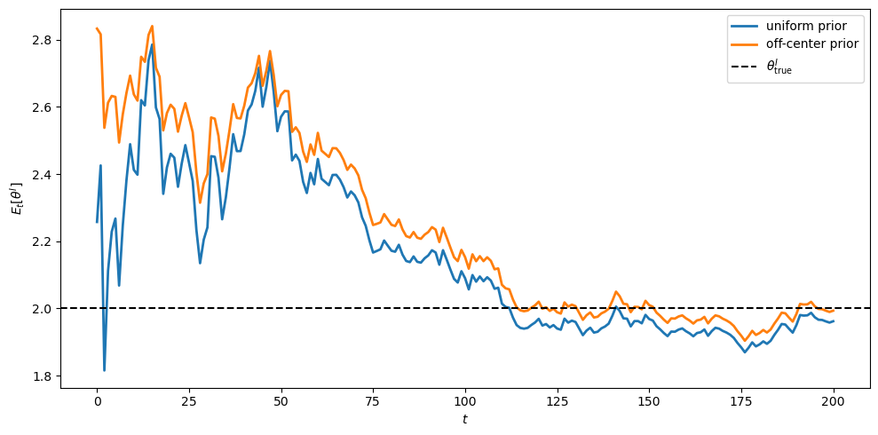
The off-center prior starts the posterior mean well above \(\theta^I_{\rm true} = 2\), but Bayesian updating drives it down to the truth.
This is the rational-learning convergence result in action: any prior that puts positive density on \(\theta^I_{\rm true}\) eventually concentrates around it.
Exercise 100.2
Speed of learning across \(\theta^I\)
Information from one period about \(\theta^I\) comes through the implied signal
The sensitivity \(|\partial s_t/\partial \theta| = \sigma^2 X^I_t/\theta^2\) depends on the level of \(\theta^I_{\rm true}\) through \(X^I_t\) and \(\theta^{-2}\).
Run the simulation for \(\theta^I_{\rm true} \in \{0.8, 2.0, 3.5\}\), holding everything else at the baseline.
Plot the posterior variance on a log scale for each case.
Which value of \(\theta^I_{\rm true}\) yields the fastest concentration, and does the result match the sensitivity formula above?
Solution
Here is one solution:
fig, ax = plt.subplots(figsize=(10, 5))
for θ_val in [0.8, 2.0, 3.5]:
    params_θ = dict(params)
    params_θ['θ_I_true'] = θ_val
    res_θ = simulate(**params_θ)
    ax.semilogy(res_θ['post_var'], lw=2,
                label=fr'$\theta^I_{{\rm true}} = {θ_val}$')
ax.set_xlabel('$t$')
ax.set_ylabel(r'${\rm Var}_t[\theta^I]$ (log scale)')
ax.legend()
plt.tight_layout()
plt.show()
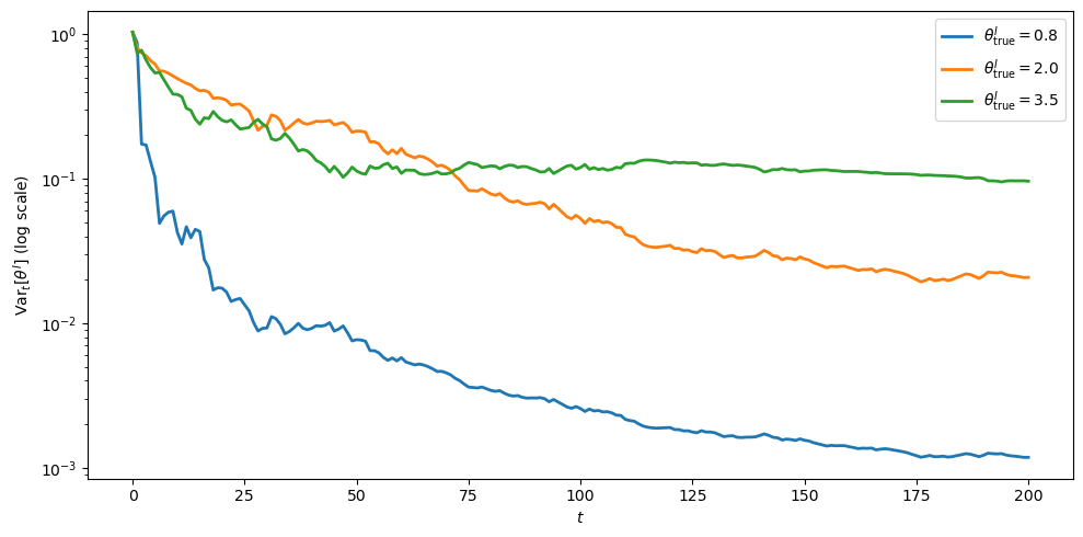
The smallest \(\theta^I_{\rm true}\) produces the steepest decline in posterior variance.
The reason is that the sensitivity \(\sigma^2 X^I_t/\theta^2\) scales as \(\theta^{-2}\) for fixed \(X^I_t\), so the same noise level conveys much more information about \(\theta^I\) when \(\theta^I\) is small.
Exercise 100.3
Effect of return noise
Larger \(\sigma^2\) widens the conditional density of \(s_t\) given \(r_t\), which one might guess slows learning.
But \(\sigma^2\) also scales the price intercept in (100.8), so price dispersion across candidate \(\theta\) grows with \(\sigma^2\).
Run the simulation with \(\sigma^2 \in \{0.25, 1.0, 4.0\}\), keeping \(\tau^2 = 1\) fixed.
Plot the posterior variance on a log scale for each \(\sigma^2\).
Explain which effect dominates in terms of the signal-to-noise ratio for inferring \(\theta^I\) from the price.
Solution
Here is one solution:
fig, ax = plt.subplots(figsize=(10, 5))
for σ2_val in [0.25, 1.0, 4.0]:
    params_σ = dict(params)
    params_σ['σ2'] = σ2_val
    res_σ = simulate(**params_σ)
    ax.semilogy(res_σ['post_var'], lw=2,
                label=fr'$\sigma^2 = {σ2_val}$')
ax.set_xlabel('$t$')
ax.set_ylabel(r'${\rm Var}_t[\theta^I]$ (log scale)')
ax.legend()
plt.tight_layout()
plt.show()
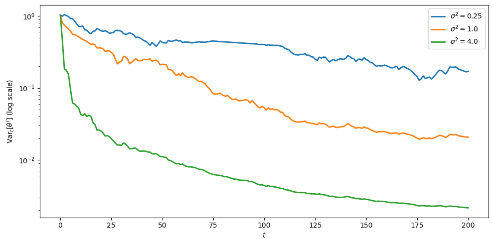
The posterior variance falls faster for larger \(\sigma^2\).
To see why, write \(\nu=\sigma^2\) and hold the realized trade \(X^I_t\) fixed.
Two nearby values of \(\theta\) imply signals separated by approximately
The likelihood compares these implied signals using \(g(s\mid r_t)\), whose conditional variance is
Thus the local signal-to-noise ratio for distinguishing nearby \(\theta\) values is proportional to
This ratio rises with \(\nu\) when \(\tau^2\) is fixed.
The price-revelation effect therefore dominates the extra return noise in this experiment.