104. Long-term Risk: An Operator Approach#
104.1. Overview#
Standard short-horizon asset pricing tells us how investors are compensated for tiny, instantaneous exposures to shocks, the short end of the term structure of risk prices.
But many of the most interesting asset pricing questions (e.g., the equity premium puzzle, the slope of the yield curve, the prices of long-dated options) concern the long end of the term structure of risk prices.
This lecture studies the long end using the operator approach of Hansen and Scheinkman [2009].
At center stage will be a stochastic discount factor process and a return process that are multiplicative across time in the sense that conditional expectations define a semigroup of valuation operators indexed by horizon \(t\).
Long-horizon behaviour of the semigroup is controlled by a single eigenvalue problem on the state space.
By solving that eigenvalue problem and selecting an appropriate eigenfunction, we can factor the multiplicative functional \(M_t\) into three economically meaningful pieces: a deterministic exponential trend, a non-negative martingale that changes probability measure, and a transient state-dependent component.
In particular, the factorization takes the form
where
\(\rho\) is a scalar (the principal eigenvalue) giving the asymptotic growth or decay rate,
\(\phi\) is a strictly positive principal eigenfunction on the state space, capturing the long-run dependence on the current state,
\(\hat M\) is a positive martingale used to change probability measure (the martingale component), and
\(\phi(X_0)/\phi(X_t)\) is a transient component that washes out as the twisted process settles into its stationary distribution.
In finite-state problems this is exactly the Perron-Frobenius decomposition of a positive matrix; in general state spaces it is a continuous-state counterpart.
We will refer to (104.1) as the multiplicative factorization associated with \((\rho,\phi,\hat M)\).
Alvarez and Jermann [2005] introduced a related permanent-transitory decomposition for stochastic discount factors.
The operator approach links that decomposition to an explicit eigenvalue problem.
See also
This lecture is closely related to the advanced lecture Additive and Multiplicative Functionals, which studies the same kind of permanent-transitory decomposition for additive and multiplicative functionals in a discrete-time linear-Gaussian setting.
Reading these two lectures together is a good way to learn about representations of long-run risks in both continuous and discrete time.
We will build up to (104.1) and use it to compute long-run risk prices in concrete models.
The plan of this lecture is to:
Set up positive multiplicative functionals \(M\) (discount factors, returns, stochastic growth) and the valuation semigroups they generate.
Introduce the generator of a semigroup, a local operator whose eigenvalue problem controls long-run behaviour.
Find the principal eigenfunction \(\phi\) and derive the factorization.
Work two examples in detail: a finite-state Markov chain (where everything reduces to Perron-Frobenius theory) and an affine diffusion model (where the eigenfunction is exponential-affine and we get closed-form formulas).
Use the factorization to compute long-run risk prices and compare them to the local risk prices appropriate for short-horizon asset pricing.
A recurring theme is that shocks to persistent state variables drive a wedge between local and long-run risk prices.
That wedge is the mechanism by which long-run risk models like Bansal and Yaron [2004] generate large equity premia.
We start with the following imports
import numpy as np
import matplotlib.pyplot as plt
from scipy.linalg import eig, expm
104.2. Multiplicative functionals#
104.2.1. Setting#
Let \(\{X_t : t \geq 0\}\) be a continuous-time Markov process with state space \(\mathcal D_0\), and let \(\mathcal F_t\) denote the filtration generated by its history.
We will work with a strong Markov process whose sample paths are càdlàg (defined below).
For the explicit formulas later we will specialize to a semimartingale that decomposes into a continuous component \(X^c\) and a pure-jump component \(X^j\):
We write the continuous-component dynamics as
and the pure-jump component as
where \(\zeta\) is the random counting measure of jumps indexed by the post-jump state \(y\), so that \(\zeta(B, [0,t])\) counts the number of jumps in \([0,t]\) landing in the Borel set \(B\).
Its compensator is \(\eta(dy \mid X_{t-})\, dt\), the rate at which \(X\) jumps from \(X_{t-}\) into a region \(dy\).
We will use this “\(y\) = post-jump state” convention throughout, matching the form \(\phi(y) - \phi(x)\) that appears in the generator below.
We also impose two simplifying assumptions:
Finite jumps on finite time intervals: only finitely many jumps occur on any bounded interval; this keeps integrals against the jump measure well-defined and finite.
Sufficient rank in \(\Gamma\) so that the Brownian shocks relevant for pricing can be recovered from the state history; this makes the Markov state \(X\) “rich enough” to describe valuation.
These assumptions let us write the generator in closed form and use martingale-based changes of measure freely.
104.2.2. Functionals and càdlàg paths#
We need a name for “a process that records something about the history of \(X\)”.
This includes, for example, a stochastic discount factor or a cumulated return.
Definition 104.1 (Functional)
A functional is a real-valued adapted process \(\{M_t : t \geq 0\}\) constructed from the history of \(X\), so that \(M_t\) is \(\mathcal F_t\)-measurable for each \(t\).
We will always work with the càdlàg version of a functional, the French acronym for “right-continuous with left limits”.
Concretely, for almost every sample path \(\omega\),
and the left limit \(M_{t-}(\omega) := \lim_{s \uparrow t} M_s(\omega)\) exists and is finite for all \(t > 0\).
Thus, paths can jump, but each jump \(\Delta M_t := M_t - M_{t-}\) occurs instantaneously.
At the jump time \(t\), the value is the post-jump value, not the pre-jump value.
Note
Why is the càdlàg property worth insisting on?
Because we will later want to (i) integrate functionals against time, (ii) apply optional stopping arguments, and (iii) take limits like \(\lim_{t \to \infty} t^{-1}\log M_t\).
All three operations need the joint measurability in \((\omega,t)\) that càdlàg paths give us automatically.
104.2.3. Multiplicativity#
The central restriction we impose on the functional \(M\) is that it is multiplicative across time.
Definition 104.2 (Multiplicative Functional)
A functional \(\{M_t : t \geq 0\}\) is multiplicative if \(M_0 = 1\) and
where \(\theta_t\) shifts the underlying Markov path forward by \(t\) units.
Why is this a useful condition to require?
Think of \(M_t = S_t\), a stochastic discount factor.
The date-\(0\) value of a date-\(t\) payoff \(\Pi_t\) is \(\mathbb{E}[S_t\Pi_t \mid \mathcal F_0]\).
If we instead buy this payoff at intermediate date \(\tau\), its date-\(\tau\) price must be
For the price to depend only on the current Markov state \(X_\tau\) (and not on the entire history up to \(\tau\)), the ratio \(S_t/S_\tau\) must be a function only of the Markov path after \(\tau\).
Thus, \(S_{\tau+u}/S_\tau = S_u(\theta_\tau)\), which is exactly (104.2).
So multiplicativity is the Markov form of the law of one price.
The same structural property is then carried over to stochastic growth and cumulated returns.
104.2.4. Additive functionals#
It is often easier to work with the log of a strictly positive multiplicative functional.
If \(M_t > 0\), we can write \(M_t = \exp(A_t)\), and the multiplicative property (104.2) becomes the corresponding additive property of \(A\).
Definition 104.3 (Additive Functional)
A functional \(\{A_t : t \geq 0\}\) is additive if \(A_0 = 0\) and
So exponentials of additive functionals are exactly the strictly positive multiplicative functionals.
In our jump-diffusion setting, a useful parameterization is
where the three functions \((\beta, \gamma, \kappa)\) play the following roles:
\(\beta(x)\) is a state-dependent drift rate ( e.g., a pure discount factor with short rate \(r(x)\) has \(\beta(x) = -r(x)\)).
\(\gamma(x)\) is a Brownian loading, controlling how Brownian shocks feed into \(A\) at state \(x\).
\(\kappa(y,x)\) is a jump amplitude that fires whenever \(X\) jumps from \(x\) to \(y\).
For everything to be well defined, we impose the natural integrability conditions
together with \(\kappa(x,x)=0\) (no jump if the state doesn’t change) and
This parameterization is rich enough for everything we do in this lecture, though additive functionals can also include things like occupation times.
104.3. Semigroups#
A multiplicative functional \(M\) together with the Markov process \(X\) defines a valuation operator for each horizon \(t\):
You should read \(\mathbb M_t \psi(x)\) as “the date-\(0\) value, starting from state \(x\), of a date-\(t\) payoff \(\psi(X_t)\)”, weighted by \(M_t\).
The family of operators \(\{\mathbb M_t\}_{t \geq 0}\) has a key compositional structure, the semigroup property.
Definition 104.4 (One-Parameter Semigroup)
A family of linear operators \(\{T_t : t \geq 0\}\) is a one-parameter semigroup if \(T_0=I\) and \(T_{t+s}=T_tT_s\) for all \(s,t \geq 0\).
It is positive if \(T_t\psi \geq 0\) whenever \(\psi \geq 0\).
Definition 104.5 (Multiplicative Semigroup)
Given a multiplicative functional \(M\), the associated multiplicative semigroup is the family of operators
The semigroup identity \(\mathbb M_{t+u} = \mathbb M_t \mathbb M_u\) follows from iterated expectations and the multiplicative property of \(M\).
Economically, this is the Markov law of iterated values: to value a date-\((t+u)\) payoff today, we can either
discount it directly from \(t+u\) back to \(0\) in one step (apply \(\mathbb M_{t+u}\)), or
first discount it from \(t+u\) back to \(t\) (apply \(\mathbb M_u\)), then discount the resulting date-\(t\) price back to \(0\) (apply \(\mathbb M_t\)).
The semigroup identity says these two procedures give the same answer.
This is the operator-level version of the intertemporal consistency that rules out arbitrage across horizons.
Four positive multiplicative functionals will appear often below.
Symbol |
Object |
Semigroup |
|---|---|---|
\(S\) |
stochastic discount factor |
\(\{\mathbb S_t\}\) |
\(V\) |
cumulated return on an asset |
\(\{\mathbb V_t\}\) |
\(G\) |
stochastic growth in cash flows |
\(\{\mathbb G_t\}\) |
\(Q=GS\) |
valuation of growing cash flows |
\(\{\mathbb Q_t\}\) |
The first three are primitives.
The fourth combines discounting and growth to value cash flows that grow stochastically over time.
Definition 104.6 (Stochastic Discount Factor)
A stochastic discount factor \(S\) is a positive multiplicative functional for which \(\mathbb{E}[S_t Z_t \mid X_0=x]\) is the date-\(0\) value of an \(\mathcal F_t\)-measurable payoff \(Z_t\).
Definition 104.7 (Valuation Functional)
Given a stochastic discount factor \(S\), a valuation functional \(V\) is a positive multiplicative functional such that \(\{V_t S_t : t \geq 0\}\) is a martingale.
Definition 104.8 (Stochastic Growth Functional)
A stochastic growth functional \(G\) is a positive multiplicative functional, interpreted as a multiplicative growth factor applied to a date-\(0\) cash flow.
Consider a cash flow \(D_t = D_0\, G_t\, \psi(X_t)\), where \(D_0 > 0\) is the date-\(0\) level and \(\psi\) is a Borel state-payoff function.
Discounting with \(S\) and growing with \(G\), its date-\(0\) value is
Definition 104.9 (Cash-Flow Valuation Semigroup)
The cash-flow valuation semigroup is the multiplicative semigroup generated by \(Q=GS\).
The long-horizon behaviour of \(\mathbb Q_t\) is the central object of the lecture: it tells us how current prices value cash-flow growth risk that materializes far in the future.
Note
The factorization \(D_t=D_0 G_t \psi(X_t)\) is not unique.
For any positive function \(\varphi\),
so a transient state-dependent factor can be shuffled between \(G\) and \(\psi\) without changing \(D_t\).
We resolve this indeterminacy by normalizing the growth component so that its permanent part is a martingale: \(G_t = \exp(\delta t)\hat G_t\), with \(\hat G\) a martingale and \(\delta\) a constant trend.
The eigenfunction construction below will tell us exactly which martingale to pick.
104.3.1. Local pricing restriction#
Before tackling long horizons, it is worth knowing what valuation looks like at the short end.
That is the standard instantaneous risk-return relation.
This will give us a benchmark against which to compare long-run risk prices.
For a textbook discrete-time treatment of the same SDF-based asset-pricing ideas, see Elementary Asset Pricing Theory.
For an estimation perspective on Euler-equation-based asset pricing, see Estimating Euler Equations by Generalized Method of Moments.
The key starting point is that a valuation functional \(V\) must satisfy the no-arbitrage requirement that \(VS\) is a martingale (Definition 104.7).
We parameterize the stochastic discount factor \(S\) and valuation functional \(V\) as additive functionals with coefficients \((\beta^s,\gamma^s,\kappa^s)\) and \((\beta^v,\gamma^v,\kappa^v)\) respectively, in the notation of (104.3).
For a generic positive multiplicative functional \(M = \exp(A)\) with parameters \((\beta,\gamma,\kappa)\), applying Itô’s formula to \(\exp(A_t)\) and requiring the drift of \(dM_t/M_{t-}\) to vanish gives the local martingale restriction:
The three terms correspond to:
the drift of \(A\) itself,
the Itô correction from the Brownian part (because \(M = e^A\) picks up a quadratic-variation contribution), and
the compensated jumps of \(M\) at the multiplier \(\exp[\kappa(y,x)]\).
We ask you to verify this in Exercise 104.4.
Applying this to \(VS\), whose parameters add: \((\beta^v + \beta^s, \gamma^v + \gamma^s, \kappa^v + \kappa^s)\), gives the local pricing restriction
This determines the drift \(\beta^v\) of any candidate valuation functional in terms of its Brownian and jump exposures.
To turn this into an expected return, note that the expected net rate of return on \(V\) is
Combining with (104.6) gives
Thus, the Brownian local risk-price vector is \(-\gamma^s(x)\), expressed in the same exposure units as \(\gamma^v(x)\).
Jump risk is priced through the function \(\kappa^s\).
This local relation is one end of the term structure of risk prices.
The eigenvalue calculations below describe the other end.
104.4. The generator#
So far we have a family of operators \(\{\mathbb M_t\}_{t \geq 0}\), one for each horizon \(t\).
That is more information than we can use directly.
What we care about is the long-run behaviour: how \(\mathbb M_t \psi\) grows as \(t \to \infty\).
The generator \(\mathbb A\) compresses the entire semigroup into one time-independent operator on the state space.
It records the instantaneous rate of change of \(M_t \psi(X_t)\), and its eigenvalues drive the long-run growth rate of \(\mathbb M_t\).
This lets us turn an asymptotic question about a family of operators into a single eigenvalue problem.
104.4.1. Discrete-time intuition#
The role of the generator is easiest to see when time is discrete, so we build the picture there once and then carry it over.
Let \(X_n\) be Markov and \(M_n\) a multiplicative functional, and define the one-period valuation operator
Iterating gives the \(n\)-period operator \(K^n\).
This parallels the logic of a transition matrix: just as \(P^n\) gives \(n\)-step probabilities, \(K^n\) weights \(n\)-period payoffs, with \(M_1\) folded in at each step.
So one local object, \(K\), controls the entire horizon-indexed family.
It also controls long-run growth: if \(K\phi = \lambda \phi\), then
so \(\lambda\) is the long-run geometric growth (or decay) rate and \(\phi\) is the long-run dependence on the current state.
The same operator gives the predictable rate of change of the weighted payoff.
By multiplicativity,
so subtracting the cumulative predictable change from the total change leaves a martingale:
Here \(K-I\) is the local rate of change of \(M_n \psi(X_n)\), and through \(K^n\) it also controls long-run growth.
104.4.2. From discrete to continuous time#
Continuous time keeps the same logic.
The natural counterpart \(K-I\) is the infinitesimal generator of the semigroup \(\{\mathbb M_t\}\), the time derivative at zero:
so that for small \(h>0\),
Note
When \(M \equiv 1\), the multiplicative semigroup reduces to the standard Markov transition semigroup \(\mathbb M_t \psi(x) = \mathbb{E}[\psi(X_t) \mid X_0=x]\), and \(\mathbb A\) becomes the familiar infinitesimal generator \(\mathcal L\) of \(X\) from textbook stochastic calculus.
For general \(M\), \(\mathbb A\) is the same kind of object but it carries extra terms that encode the instantaneous “yield” of \(M\): discount rates, Brownian risk prices, jump multipliers.
That is exactly what we will see when we write down its closed form in (104.8) below.
Why is this the right object?
If \(\mathbb A\phi = \rho\phi\), then the candidate
is automatically a local martingale.
When \(\hat M\) is in fact a martingale (the content of Assumption 6.1 in Hansen and Scheinkman [2009]), taking expectations gives the continuous-time analogue of \(K^n\phi = \lambda^n\phi\):
Without that upgrade we get only the supermartingale inequality \(\mathbb M_t \phi \le \exp(\rho t)\, \phi\), which we will revisit below.
So the long-run behaviour of \(\mathbb M_t\) is encoded in an eigenvalue problem for the local operator \(\mathbb A\), together with the martingale property of \(\hat M\).
104.4.3. Extended generator#
The limit definition above needs a qualification.
To make the limit \(h \downarrow 0\) rigorous, the textbook definition requires \((\mathbb M_h\psi - \psi)/h\) to converge to \(\mathbb A\psi\) in a chosen norm, typically uniform convergence over bounded continuous functions, where the semigroup is a contraction.
But the functions we care about most are the principal eigenfunctions \(\phi\) solving \(\mathbb A\phi = \rho\phi\), and these typically grow with the state \(X\) (in the affine-Gaussian benchmark, \(\phi\) is exponential-affine in \(x\)).
So they do not lie in this space, and the limit need not converge for them.
Hansen and Scheinkman [2009] sidestep this by characterizing \(\mathbb A\) through a Doob-Meyer style semimartingale decomposition of \(M_t \psi(X_t)\), a pathwise condition that does not require any norm.
This is the continuous-time counterpart to writing \(K - I\) as the predictable rate of change of \(M_n\psi(X_n)\) in discrete time.
The resulting extended generator admits unbounded \(\psi\), has a strictly larger domain than the textbook generator, and agrees with it where both are defined.
Concretely:
Definition 104.10 (Extended Generator)
Fix a Borel function \(\psi\), and look for a second Borel function \(\chi\) that will play the role of “the instantaneous rate of change of \(M_t \psi(X_t)\) at the current state”. We ask whether there exists \(\chi\) such that
is a local martingale.
We then say \(\psi\) lies in the domain of the extended generator \(\mathbb A\) of \(M\), and we define the operator by
The three terms play the same roles as in discrete time:
\(M_t \psi(X_t) - \psi(X_0)\) is the total change in the weighted payoff over \([0, t]\),
\(\int_0^t M_s \chi(X_s)\, ds\) accumulates the expected rate of change along the path,
\(N_t\) is the residual.
Requiring \(N_t\) to be a local martingale pins down \(\chi = \mathbb A\psi\) as the instantaneous expected rate of change of \(M_t \psi(X_t)\) at the current state.
When \(M \equiv 1\), the definition reduces to Dynkin’s formula for the standard Markov generator \(\mathcal L \psi(x) = \lim_{t \downarrow 0} t^{-1}\bigl[\mathbb{E}\psi(X_t) - \psi(x)\bigr]\).
When \(X\) is a jump diffusion, Itô’s formula applied to \(M_t\psi(X_t)\) produces the closed-form expression for \(\mathbb A\psi\) in (104.8) below.
104.4.4. A closed form for jump diffusions#
For the jump-diffusion setting introduced above, we can compute \(\mathbb A\) explicitly by applying Itô’s formula to \(M_t\phi(X_t)\).
Suppose the continuous part of \(X\) satisfies
with diffusion matrix \(\Sigma = \Gamma \Gamma^\top\), and let \(\eta(dy \mid x)\) denote the jump compensator.
If \(M=\exp(A)\) is parameterized by \((\beta,\gamma,\kappa)\) as in (104.3), then for smooth \(\phi\),
The four terms have transparent interpretations:
The first term is the standard Markov drift, modified by \(\Gamma\gamma\), a covariance correction between the Brownian shocks driving \(X\) and those driving \(M\).
The second is the standard diffusion (Itô) term.
The third integrates \(\phi\) against the jump-compensated transition rates, reweighted by the jump multiplier \(\exp[\kappa(y,x)]\).
The fourth is a multiplicative yield-like term that multiplies \(\phi(x)\) itself and combines the drift of \(M\), the Brownian Itô correction, and the compensated jumps.
Note
When \(M=S\) is a stochastic discount factor, the local risk prices are spread across the four pieces of the generator rather than concentrated in the level term.
Brownian factor prices enter through the drift modification \(\xi \to \xi + \Gamma\gamma\) in the first line.
Jump-risk prices enter through the tilted jump measure \(\eta \to \exp[\kappa]\,\eta\) in the third line.
The level term in the fourth line contains the instantaneous risk-free rate component (the short end of the term structure) plus the jump-compensator contribution \(\int(\exp[\kappa]-1)\,\eta\).
We ask readers to verify the derivation of (104.8) in Exercise 104.5.
We will apply this formula directly in the affine-diffusion example below.
104.5. Principal eigenfunctions#
We now arrive at the central technical question of the lecture:
Which positive payoffs grow at a constant proportional rate under the valuation semigroup?
The answer, when it exists, is a positive eigenfunction of the generator.
Definition 104.11 (Eigenfunction of the Extended Generator)
A Borel function \(\phi\) is an eigenfunction of \(\mathbb A\) with eigenvalue \(\rho\) if
A principal eigenfunction is an eigenfunction \(\phi\) that is strictly positive on the state space: \(\phi(x) > 0\) for all \(x \in \mathcal D_0\).
The strict-positivity requirement matters because \(\phi\) will appear in denominators throughout: it has to be safe to divide by it.
104.5.1. From eigenfunction to factorization#
Why does an eigenfunction of \(\mathbb A\) give us the multiplicative factorization (104.1)?
The discrete-time analogy points the way. If \(K\phi = \lambda\phi\), then
is a martingale: the eigenvalue equation absorbs the one-step drift of \(M_n\phi(X_n)\) exactly.
In continuous time, \(\lambda^n\) becomes \(\exp(\rho t)\), and the candidate martingale is
Let’s check that \(\hat M\) is indeed a local martingale.
By the definition of \(\mathbb A\), the semimartingale \(Z_t := M_t\phi(X_t)\) admits the decomposition
where \(N\) is a local martingale.
The eigenvalue equation \(\mathbb A\phi = \rho\phi\) replaces the drift by \(\rho Z_t\, dt\), and integration by parts gives
So \(\exp(-\rho t) Z_t\) is a local martingale, and dividing by \(\phi(X_0)\) shows the same for \(\hat M\).
Rearranging (104.10) for \(M_t\) recovers the factorization (104.1), with \(\hat M\) in the role of the martingale component.
Definition 104.12 (Martingale Component and Twisted Measure)
When \(\hat M\) is a martingale (not merely a local martingale), it is the martingale component associated with \((\rho,\phi)\) and defines the twisted probability measure by weighting date-\(t\) events with \(\hat M_t\):
The verification establishes only that \(\hat M\) is a local martingale, but the definition above (and the change-of-measure interpretation of \(\hat M\)) both require it to be a martingale.
We close this gap by adopting Assumption 6.1 of Hansen and Scheinkman [2009]:
The local martingale \(\hat M\) defined in (104.10) is a martingale, i.e. \(\mathbb{E}[\hat M_t \mid X_0 = x] = 1\) for every \(t \geq 0\) and \(x\).
We carry this assumption from here on.
Even without closing the gap we still get one-sided control.
Since \(\hat M\) is nonnegative with \(\hat M_0 = 1\), it is a supermartingale, so \(\mathbb{E}[\hat M_t \mid X_0=x] \leq 1\).
Taking expectations in (104.10),
so \(\rho\) is at least an upper bound on the long-run growth rate of \(\mathbb M_t \phi\).
When \(\hat M\) is in fact a martingale, \(\mathbb{E}[\hat M_t] = 1\), the inequality becomes an equality, and the local condition \(\mathbb A\phi = \rho\phi\) lifts to the semigroup eigenvalue equation
104.5.2. Stability of the twisted process#
We now have a factorization (104.1) for any principal eigenfunction.
But for \((\rho,\phi)\) to describe long-run behaviour of \(\mathbb M_t\) the twisted process must settle into a stationary regime as \(t \to \infty\).
If it doesn’t, the transient factor \(\phi(X_0)/\phi(X_t)\) will not vanish, and we cannot read off the asymptotics from \(\rho\) alone.
We need three conditions, each ruling out a specific way in which the twisted process can fail to settle down.
Let \(\hat E\) and \(\widehat{\Pr}\) denote expectation and probability under the twisted measure, and let \(\hat{\mathbb A}\) be the generator of \(X\) under that measure.
Condition 1: a stationary distribution exists.
Definition 104.13 (Stationary Distribution of the Twisted Process)
A probability measure \(\hat\varsigma\) on \(\mathcal D_0\) is a stationary distribution for the twisted process if
for every \(\psi\) in the \(L^\infty\) domain of \(\hat{\mathbb A}\).
\(\hat\varsigma\) is the candidate long-run distribution.
Without it, the twisted process has no steady state, and the long-run limit cannot be expressed as a state-space integral.
Condition 2: every important region is reachable.
Definition 104.14 (Irreducible Skeleton)
The discretely sampled skeleton \(\{X_{\Delta j} : j = 0, 1, \ldots\}\) is irreducible relative to \(\hat\varsigma\) if there exists \(\Delta > 0\) such that, for every Borel set \(\Lambda \subseteq \mathcal D_0\) with \(\hat\varsigma(\Lambda) > 0\),
Without it, the long-run distribution could depend on the starting state; different basins of attraction would give different limits.
Condition 3: every important region is visited infinitely often.
Definition 104.15 (Harris Recurrence)
The process \(X\) is Harris recurrent under the twisted measure if, for every Borel set \(\Lambda \subseteq \mathcal D_0\) with \(\hat\varsigma(\Lambda) > 0\),
Reachability (Condition 2) is not enough.
A set may be reachable but visited with vanishingly small probability, so time averages fail to converge to \(\hat\varsigma\)-averages.
Harris recurrence is the continuous-state counterpart to a “recurrent state” in a finite chain.
Collecting the three conditions:
Definition 104.16 (Stochastically Stable Twisted Process)
The \(\hat M\)-twisted Markov process is stochastically stable if it has a stationary distribution \(\hat\varsigma\), the skeleton \(\{X_{\Delta j}\}\) is irreducible relative to \(\hat\varsigma\), and \(X\) is Harris recurrent under the twisted measure.
104.5.3. The long-run approximation#
Under the martingale condition for \(\hat M\), strict positivity of \(M\), and stochastic stability, the long-run limit takes a clean form:
Read this as follows:
The factor \(\exp(\rho t)\) captures the exponential growth or decay of the semigroup; once we divide it out, what remains has a finite limit.
The state dependence in that limit is entirely captured by \(\phi(x)\).
The scalar \(\int (\psi/\phi)\, d\hat\varsigma\) is the long-run intensity of the payoff \(\psi\), weighted by \(1/\phi\) and averaged against the twisted stationary distribution.
The two precise cases of Proposition 7.1 of Hansen and Scheinkman [2009] are:
Sampled grid, \(\hat\varsigma\)-almost every starting state. Fix any \(\Delta>0\) and assume \(\int |\psi|/\phi\, d\hat\varsigma < \infty\); then the limit holds along \(t = \Delta j\) for \(\hat\varsigma\)-almost every \(x \in \mathcal D_0\).
Continuous \(t\), every starting state. If \(\psi/\phi\) is bounded then the limit holds for every \(x \in \mathcal D_0\) and every \(t \to \infty\), with no continuity assumption on \(\psi\).
Note
There can be more than one positive eigenfunction of \(\mathbb A\) for which the associated \(\hat M\) is a martingale, possibly with different eigenvalues.
Stochastic stability selects a particular one.
By Proposition 7.2 of Hansen and Scheinkman [2009], the stable eigenfunction’s eigenvalue \(\rho\) is the smallest among all eigenvalues of \(\mathbb A\) that admit a strictly positive eigenfunction satisfying the maintained conditions.
Any other positive eigenfunction sharing this \(\rho\) is proportional to \(\phi\) \(\hat\varsigma\)-almost surely.
The finite-state section below states the same selection in the more familiar Perron-Frobenius language, calling \(\rho\) the eigenvalue with the largest real part among all eigenvalues of \(A\).
These two descriptions identify the same eigenvalue because in the irreducible finite-state case only one eigenvalue of \(A\) admits a strictly positive eigenvector.
In the affine example below the two sets pull apart, since the quadratic (104.18) has two roots \(c_f\) that both give strictly positive exponential-affine eigenfunctions with distinct eigenvalues.
Stochastic stability picks the smaller \(\rho\) by rejecting the root that produces an explosive twisted process.
104.6. A finite-state Markov chain#
We now apply the framework to a concrete example.
We start with the simplest case: a finite-state Markov chain.
For background on finite Markov chains in discrete time, see Finite Markov Chains.
For the asset-pricing applications of finite-state chains that motivate the construction here, see Asset Pricing: Finite State Models.
Here, every abstract object collapses to a familiar one:
Abstract object |
Finite-state version |
|---|---|
Markov process \(X\) |
continuous-time chain with intensity matrix \(U\) |
Generator \(\mathbb A\) |
a matrix \(A\) |
Semigroup \(\mathbb M_t\) |
matrix exponential \(\exp(tA)\) |
Principal eigenfunction \(\phi\) |
Perron right eigenvector |
Principal eigenvalue \(\rho\) |
dominant real eigenvalue of \(A\) |
Stationary distribution \(\hat\varsigma\) |
left eigenvector of twisted generator |
So the long-run analysis reduces to Perron-Frobenius theory.
(For an introduction to the Perron-Frobenius theorem, see The Perron-Frobenius Theorem.)
104.6.1. Setup#
Let \(X\) take values in \(\{x_1,\ldots,x_N\}\) and let \(U\) be its intensity matrix.
Definition 104.17 (Intensity Matrix)
An intensity matrix \(U\) for a finite-state continuous-time Markov chain satisfies \(u_{ij} \geq 0\) for \(i \neq j\) and \(\sum_j u_{ij}=0\) for each state \(i\).
Off-diagonal entries \(u_{ij}\) are the jump rates from state \(i\) to state \(j\); the diagonal entry \(u_{ii} = -\sum_{j \neq i}u_{ij}\) is minus the exit rate from state \(i\).
Let the multiplicative functional have
a discount or decay rate \(r_i\) in state \(i\) (the analogue of the drift \(\beta(X_s)\) in the additive parameterization), and
a jump multiplier \(\exp[\kappa(x_j,x_i)]\) that fires whenever the state jumps from \(i\) to \(j\).
In code below, κ[j, i] means \(\kappa(x_j,x_i)\).
Then the generator matrix \(A\) for the multiplicative semigroup is
The off-diagonal entries are the chain’s jump rates weighted by the jump multipliers; the diagonal entries combine the exit rate with the in-state decay rate.
The semigroup is then just \(\mathbb M_t = \exp(tA)\).
For an irreducible chain with strictly positive jump multipliers, the principal eigenvalue \(\rho\) is the unique real eigenvalue of \(A\) with largest real part, and the associated right eigenvector is strictly positive.
The twisted generator under the principal eigenpair \((\rho,\phi)\) is
where \(D_\phi = \operatorname{diag}(\phi)\).
The row sums of \(\hat A\) vanish, so \(\hat A\) is itself a valid intensity matrix.
The stationary distribution \(\hat\varsigma\) solves \(\hat\varsigma^\top \hat A = 0\).
The helper functions below implement these three calculations.
def build_generator(U, r, κ):
    """Generator matrix for a finite-state multiplicative semigroup.

    κ[j, i] is the log jump multiplier for a transition i -> j.
    """
    U = np.asarray(U, dtype=float)
    r = np.asarray(r, dtype=float)
    κ = np.asarray(κ, dtype=float)

    A = U * np.exp(κ.T)
    np.fill_diagonal(A, np.diag(U) - r)
    return A


def principal_eigenpair(A):
    """Perron eigenpair with a positive right eigenvector."""
    vals, vecs = eig(A)
    idx = np.argmax(vals.real)

    ρ = vals[idx].real
    φ = vecs[:, idx].real

    if φ.sum() < 0:
        φ = -φ

    if np.any(φ <= 0):
        if np.min(φ) > -1e-10:
            φ = np.maximum(φ, 0)
        else:
            raise ValueError(
                "Dominant eigenvector is not strictly positive.")

    φ = φ / φ.mean()
    return ρ, φ


def twisted_generator(A, ρ, φ):
    """Generator under the twisted measure."""
    D = np.diag(φ)
    D_inv = np.diag(1 / φ)
    return D_inv @ A @ D - ρ * np.eye(len(φ))


def stationary_distribution(Q):
    """Stationary distribution of a finite-state generator."""
    vals, vecs = eig(Q.T)
    idx = np.argmin(np.abs(vals))
    π = vecs[:, idx].real

    if π.sum() < 0:
        π = -π

    π = np.maximum(π, 0)
    return π / π.sum()
104.6.2. Two states#
Consider a boom-recession economy.
State 1 is a boom (higher short rate \(r_1=0.05\), switching to recession at rate \(\lambda_1 = 0.30\)).
State 2 is a recession (lower short rate \(r_2=0.02\), switching to boom at rate \(\lambda_2 = 0.50\)).
For now we set the jump multipliers to zero, so the SDF only changes continuously through the in-state decay rates.
λ_1 = 0.30
λ_2 = 0.50

U = np.array([[-λ_1,  λ_1],
              [ λ_2, -λ_2]])

r = np.array([0.05, 0.02])
κ = np.zeros((2, 2))

A = build_generator(U, r, κ)
ρ, φ = principal_eigenpair(A)

print("A =")
print(np.round(A, 4))
print(f"\nρ = {ρ:.6f}")
print(f"φ = {φ}")
print(f"long-run zero-coupon yield = {-ρ:.4f}")
A =
[[-0.35  0.3 ]
 [ 0.5  -0.52]]

ρ = -0.038484
φ = [0.98116799 1.01883201]
long-run zero-coupon yield = 0.0385
Note that \(-\rho\) is the asymptotic yield on a zero-coupon bond: from (104.1), the date-\(0\) price of a long zero-coupon bond decays like \(\exp(\rho t)\), so its yield is \(-\rho\).
Let’s verify the semigroup eigenvalue equation \(\mathbb M_t \phi = \exp(\rho t)\phi\) numerically.
for t in [1.0, 5.0, 25.0]:
    lhs = expm(t * A) @ φ
    rhs = np.exp(ρ * t) * φ
    err = np.max(np.abs(lhs - rhs))
    print(f"t = {t:4.1f}, error = {err:.2e}")
t =  1.0, error = 1.11e-16
t =  5.0, error = 4.44e-16
t = 25.0, error = 1.67e-16
The error is at machine precision for every \(t\), so the equation holds exactly up to floating-point noise from the eigendecomposition.
Next we compute the twisted generator \(\hat A\) and the stationary distribution \(\hat\varsigma\) of the chain under the twisted measure.
This is the candidate long-run distribution that appears in the long-run limit (104.12).
A_hat = twisted_generator(A, ρ, φ)
ς_hat = stationary_distribution(A_hat)

print("twisted generator row sums:")
print(np.round(A_hat.sum(axis=1), 12))

print("\ntwisted stationary distribution:")
print(f"  boom      {ς_hat[0]:.4f}")
print(f"  recession {ς_hat[1]:.4f}")
twisted generator row sums:
[-0.  0.]

twisted stationary distribution:
  boom      0.6072
  recession 0.3928
This twisted stationary distribution (not the original chain’s stationary distribution) is what determines long-horizon valuations.
It differs from the stationary distribution of the original chain because the eigenfunction \(\phi\) reweights states by how persistently they affect the multiplicative functional.
For any payoff function \(\psi\), the long-run limit (104.12) is the vector
Let’s check that the rescaled semigroup converges to this limit as \(t\) grows.
ψ = np.array([1.0, 2.0])
limit = φ * np.sum((ψ / φ) * ς_hat)

for t in [1, 5, 20, 80]:
    approx = np.exp(-ρ * t) * expm(t * A) @ ψ
    print(f"t = {t:2d}, normalized value = {approx}")

print("\nlimit =", limit)
t =  1, normalized value = [1.19917652 1.68031101]
t =  5, normalized value = [1.35687434 1.42719756]
t = 20, normalized value = [1.36377325 1.41612444]
t = 80, normalized value = [1.3637733  1.41612436]

limit = [1.3637733  1.41612436]
The numerical values converge to the limit; the next plot shows the same convergence pictorially.
t_grid = np.linspace(0.01, 80, 400)
rescaled = np.array([np.exp(-ρ * t) * expm(t * A) @ ψ for t in t_grid])

fig, ax = plt.subplots()
ax.plot(t_grid, rescaled[:, 0], lw=2, label="starting from boom")
ax.plot(t_grid, rescaled[:, 1], lw=2, label="starting from recession")
ax.axhline(limit[0], color="C0", ls="--", lw=1, alpha=0.7)
ax.axhline(limit[1], color="C1", ls="--", lw=1, alpha=0.7)
ax.set_xlabel("$t$")
ax.set_ylabel(r"$e^{-\rho t}\,(\mathbb{M}_t \psi)(x)$")
ax.legend()
plt.show()
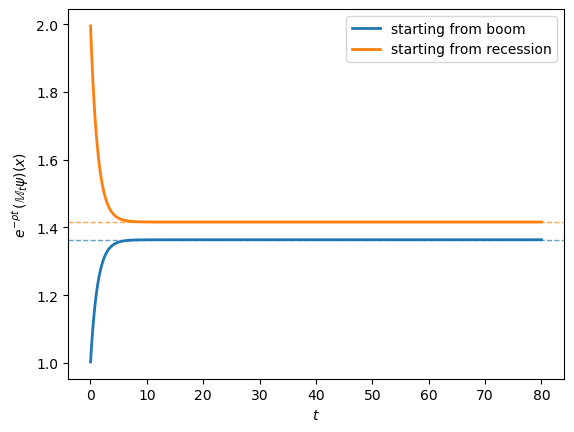
Fig. 104.1 Convergence of the rescaled semigroup to its long-run limit#
The two solid curves trace the rescaled values starting from each state, and the dashed horizontal lines mark the limits predicted by (104.12).
Both curves settle onto their predicted limits, confirming that the long-run behaviour depends on the starting state only through \(\phi\).
Note
The asymptotic exponential rate of convergence is governed by the gap between the real part of the leading eigenvalue \(\rho\) and the largest real part among the remaining eigenvalues of \(A\).
For an irreducible Metzler matrix the leading eigenvalue is real and its real part is strictly larger than the others, so this gap is well defined.
Exercise 104.3 works through a three-state example where the gap can be checked directly.
104.6.3. Adding jumps#
State transitions in this chain are discontinuous, so it is natural to allow the multiplicative functional to jump at the transition times.
These jumps are the analogue of the \(\kappa\) function in the jump-diffusion parameterization.
A natural example arises with a stochastic discount factor that jumps down when the economy moves from recession into boom and up on the reverse transition.
The matrix κ_jump below encodes this.
We use the convention
κ[j, i] = log jump multiplier of \(M\) for the transition \(i \to j\), with
state index 0 = boom and state index 1 = recession.
# recession (1) -> boom (0): SDF jumps down on good news (exp(-0.20))
# boom (0) -> recession (1): SDF jumps up on bad news (exp(+0.30))
κ_jump = np.array([[ 0.0, -0.20],
                   [ 0.30,  0.0]])

A_jump = build_generator(U, r, κ_jump)
ρ_jump, φ_jump = principal_eigenpair(A_jump)

print(f"ρ without jumps = {ρ:.6f}")
print(f"ρ with jumps    = {ρ_jump:.6f}")
print("\nφ with jumps:")
print(φ_jump)
ρ without jumps = -0.038484
ρ with jumps    = -0.019067

φ with jumps:
[1.10059123 0.89940877]
To see how the long-run rate \(\rho\) responds to jump risk, we hold the boom-to-recession multiplier fixed and trace out \(\rho\) as the recession-to-boom multiplier varies.
κ_grid = np.linspace(-0.5, 0.5, 100)
ρ_grid = np.empty_like(κ_grid)

for n, k in enumerate(κ_grid):
    κ_temp = np.array([[0.0, k],
                       [0.30, 0.0]])
    A_temp = build_generator(U, r, κ_temp)
    ρ_grid[n], _ = principal_eigenpair(A_temp)

fig, ax = plt.subplots()
ax.plot(κ_grid, ρ_grid, lw=2)
ax.axhline(ρ, color="black", ls="--", lw=1)
ax.axvline(0, color="black", ls=":", lw=1)
ax.set_xlabel("jump log multiplier for recession to boom")
ax.set_ylabel("principal eigenvalue")
plt.show()
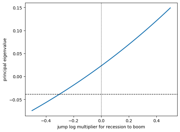
Fig. 104.2 Jumps and the long-run growth rate#
The principal eigenvalue is monotonically increasing in the recession-to-boom log multiplier: as that multiplier rises, \(M\) jumps less downward (or more upward) on good news, which mechanically pushes \(\rho\) up.
The economically sensible SDF region is to the left of zero, where the multiplier is negative.
104.7. The affine diffusion example#
We now move to a continuous-state model.
We will use a two-factor affine specification that captures the two main empirical features of asset returns:
stochastic volatility, where the dispersion of shocks is itself a state variable, and
predictable growth, where a small, persistent state variable shifts expected growth rates.
This is the kind of state process used in long-run risk models like Bansal and Yaron [2004].
We work with two independent state components: a Feller square-root process \(X^f\) (stochastic volatility) and an Ornstein-Uhlenbeck process \(X^o\) (predictable growth):
The parameters \(\xi_f, \xi_o>0\) are mean-reversion speeds, \(\bar x_f, \bar x_o\) are the unconditional means, and \(\sigma_f, \sigma_o\) are diffusion coefficients.
The OU process \(X^o\) is the continuous-time analogue of the AR(1) process studied in AR(1) Processes, and continuous-time linear asset-pricing models in the same family are developed in Affine Models of Asset Prices.
We follow a sign convention with \(\sigma_o>0\) and \(\sigma_f<0\): a positive \(B^f\) shock then reduces volatility, in line with the empirical “leverage effect.”
Now consider a multiplicative functional \(M=\exp(A)\) with affine parameters:
So the drift of \(A\) is affine in the state (\(\bar\beta + \beta_f X^f + \beta_o X^o\)), the Brownian loadings are constant in the \(B^o\) direction and proportional to \(\sqrt{X^f}\) in the \(B^f\) direction.
104.7.1. Why exponential-affine eigenfunctions work#
When the state is affine and the drift of \(A\) is affine, applying the generator to an exponential-affine function \(\phi(x^f,x^o) = \exp(c_f x^f + c_o x^o)\) returns another exponential-affine function.
This closure property turns the eigenvalue equation \(\mathbb A\phi = \rho\phi\) into a small system of algebraic equations in \((c_f, c_o, \rho)\).
Definition 104.18 (Exponential-Affine Eigenfunction)
An eigenfunction \(\phi\) of \(\mathbb A\) on a state space \(\mathcal D_0 \subseteq \mathbb R^n\) is exponential-affine if
for some constant \(c_0 \in \mathbb R\) and vector \(c \in \mathbb R^n\).
Substituting \(\phi(x^f,x^o) = \exp(c_f x^f + c_o x^o)\) into the generator formula (104.8) and matching coefficients of \(x^f\), \(x^o\), and the constant term gives
and
The two candidate values for \(c_f\) are
The eigenvalue is then determined by matching the constant term:
Equation (104.18) gives two candidate values of \(c_f\), and we need to know which one is the principal eigenfunction.
This is where stochastic stability (Definition 104.16) does real work.
Under the twisted measure, the drift of \(X^f\) is
so the mean-reversion coefficient becomes
If this is positive, the twisted square-root process stays stationary; if it is negative, the twisted process is explosive and the eigenfunction is not the long-run-relevant one.
So we pick the root that keeps the twisted process mean-reverting, exactly the way stochastic stability selects the principal eigenfunction in the abstract theory.
def solve_affine_eigenfunction(params):
    """Solve the exponential-affine eigenvalue problem."""
    ξ_f = params["ξ_f"]
    xbar_f = params["xbar_f"]
    σ_f = params["σ_f"]
    ξ_o = params["ξ_o"]
    xbar_o = params["xbar_o"]
    σ_o = params["σ_o"]
    β_bar = params["β_bar"]
    β_f = params["β_f"]
    β_o = params["β_o"]
    γ_f = params["γ_f"]
    γ_o = params["γ_o"]

    co = β_o / ξ_o

    disc = ((ξ_f - γ_f * σ_f) ** 2
            - σ_f ** 2 * (2 * β_f + γ_f ** 2))

    if disc < 0:
        raise ValueError("No real affine eigenfunction for these parameters.")

    root = np.sqrt(disc)
    cf_roots = (
        ((ξ_f - γ_f * σ_f) - root) / σ_f ** 2,
        ((ξ_f - γ_f * σ_f) + root) / σ_f ** 2
    )

    def mean_reversion(cf):
        return ξ_f - σ_f * (γ_f + cf * σ_f)

    for cf in cf_roots:
        mr = mean_reversion(cf)
        if mr > 0:
            break
    else:
        raise ValueError("Neither root gives a stationary twisted process.")

    ρ = (β_bar
         + γ_o ** 2 / 2
         + cf * ξ_f * xbar_f
         + co * (ξ_o * xbar_o + γ_o * σ_o)
         + co ** 2 * σ_o ** 2 / 2)

    return cf, co, ρ, mr
104.7.2. A Breeden SDF#
To make things concrete, we now plug in a specific stochastic discount factor: the Breeden CRRA consumption-based SDF.
Breeden [1979] derived the continuous-time SDF for an investor with time-separable CRRA preferences over a consumption stream.
We specify log consumption with the same affine state \(X^o\) driving expected growth and \(\sqrt{X^f}\) driving volatility:
With time-separable CRRA utility (risk aversion \(a\)) and subjective discount rate \(b\), the stochastic discount factor is
i.e. an exponential of \(-b\) times time minus \(a\) times log consumption growth.
Reading off the additive functional coefficients gives
We will use these parameters in the numerical example below.
104.7.3. Recursive preferences (optional)#
A famous limitation of CRRA preferences is that they conflate risk aversion with the elasticity of intertemporal substitution.
Recursive preferences Epstein and Zin [1989], Kreps and Porteus [1978] separate the two, and add a forward-looking continuation-value term to the discount-factor expression.
This is what powers the equity-premium results in Bansal and Yaron [2004].
A QuantEcon lecture that studies long-run dynamics under recursive preferences in a different setting is Survival and Long-Run Dynamics under Recursive Preferences.
This section derives the SDF coefficients for the unit-elasticity recursive specification.
You can skip on a first read and come back later — the numerical example uses the simpler Breeden parameters above.
For the unit-elasticity recursive specification, conjecture a continuation value of the form
Matching the local mean of this continuation value gives
The relevant solution has \(w_o=1/(\xi_o+b)\), selects the stable root of the quadratic for \(w_f\), and then determines \(\bar w\) from the constant equation.
The stochastic discount factor is the product \(S_t=\exp(A_t^B)\exp(A_t^W)\), where the Breeden-like logarithmic component is
The continuation-value martingale component is
Thus the recursive-utility SDF has affine parameters
The local Brownian risk prices are therefore \(\sqrt{x^f}[a\vartheta_f+(a-1)w_f\sigma_f]\) for \(B^f\) exposure and \(a\vartheta_o+(a-1)w_o\sigma_o\) for \(B^o\) exposure.
The numerical example below uses the simpler Breeden specification, but the same operator calculation applies once the SDF parameters are replaced by (104.24).
104.7.4. Numerical example#
Let’s set up parameters and solve for the principal eigenpair.
We use parameters in the standard long-run-risk neighbourhood: a mean-reverting volatility factor \(X^f\) with mean \(0.04\), a slower-moving predictable-growth factor \(X^o\) with mean \(0.02\), risk aversion \(a=4\), and a time discount rate \(b=0.03\).
params_state = {
    "ξ_f": 0.70,
    "xbar_f": 0.04,
    "σ_f": -0.20,
    "ξ_o": 0.50,
    "xbar_o": 0.02,
    "σ_o": 0.01,
}

a = 4.0
b = 0.03
ϑ_f = 0.06
ϑ_o = 0.02

params_sdf = {
    **params_state,
    "β_bar": -b,
    "β_f": 0.0,
    "β_o": -a,
    "γ_f": -a * ϑ_f,
    "γ_o": -a * ϑ_o,
}

cf_s, co_s, ρ_s, mr_s = solve_affine_eigenfunction(params_sdf)

print("principal eigenfunction φ(xf, xo) = exp(cf xf + co xo)")
print(f"cf = {cf_s:.6f}")
print(f"co = {co_s:.6f}")
print(f"ρ = {ρ_s:.6f}")
print(f"twisted mean-reversion coefficient for Xf = {mr_s:.6f}")
print(f"long-run zero-coupon yield = {-ρ_s:.4f}")
principal eigenfunction φ(xf, xo) = exp(cf xf + co xo)
cf = 0.044232
co = -8.000000
ρ = -0.095962
twisted mean-reversion coefficient for Xf = 0.650231
long-run zero-coupon yield = 0.0960
The long-run zero-coupon yield \(-\rho_s\) represents the asymptotic decay rate in the SDF expectation \(\mathbb{E}[S_t]\).
We can also check that the rejected root for \(c_f\) would have produced a non-stationary twisted process, a clear example of stochastic stability selecting one of two algebraically valid eigenfunctions.
ξ_f = params_sdf["ξ_f"]
σ_f = params_sdf["σ_f"]
γ_f = params_sdf["γ_f"]
β_f = params_sdf["β_f"]

disc = ((ξ_f - γ_f * σ_f) ** 2
        - σ_f ** 2 * (2 * β_f + γ_f ** 2))
root = np.sqrt(disc)

cf_candidates = np.array([
    ((ξ_f - γ_f * σ_f) - root) / σ_f ** 2,
    ((ξ_f - γ_f * σ_f) + root) / σ_f ** 2
])

for cf in cf_candidates:
    mr = ξ_f - σ_f * (γ_f + cf * σ_f)
    print(f"cf = {cf:8.4f}, twisted mean reversion = {mr:8.4f}")
cf =   0.0442, twisted mean reversion =   0.6502
cf =  32.5558, twisted mean reversion =  -0.6502
104.7.5. The martingale component#
Now that we have the eigenpair \((\rho,\phi)\), we can write down all three pieces of the factorization (104.1) explicitly.
The martingale component \(\hat M_t = \exp(\hat A_t)\) defined in (104.10) has log
The first line is the Brownian integral (the “exponential martingale” piece); the second is the Itô correction needed to make it a martingale.
Under the twisted measure induced by \(\hat M\), the drifts of the state variables shift to
The drift distortions are exactly the Girsanov shifts induced by the Brownian loadings of \(\hat M\).
Let’s now simulate the state and check the factorization numerically.
The first check is the algebraic identity: once we define \(\hat M\) through (104.10), the equation \(M_t = \exp(\rho t)\hat M_t \phi(X_0)/\phi(X_t)\) is automatic for any choice of \((\rho,\phi)\), and the error below is just floating-point round-off.
The second, substantive, check is whether the eigenpair \((\rho,\phi)\) we solved for really makes \(\hat M\) a martingale, which we approximate by computing \(\mathbb{E}[\hat M_t]\) across many simulated paths.
def brownian_increments(n, dt, seed=1234):
    """Independent Brownian increments for the simulation."""
    rng = np.random.default_rng(seed)
    draws = rng.normal(scale=np.sqrt(dt), size=(n, 2))
    return draws[:, 0], draws[:, 1]


def simulate_states(params, T=40.0, dt=0.01, seed=1234):
    """Euler simulation of the affine state process."""
    n = int(T / dt)
    t = np.linspace(0, T, n + 1)
    Xf = np.empty(n + 1)
    Xo = np.empty(n + 1)
    dBf, dBo = brownian_increments(n, dt, seed)

    Xf[0] = params["xbar_f"]
    Xo[0] = params["xbar_o"]

    for k, (dBf_k, dBo_k) in enumerate(zip(dBf, dBo)):
        xf = max(Xf[k], 1e-10)
        xo = Xo[k]

        Xf[k + 1] = (xf
                     + params["ξ_f"] * (params["xbar_f"] - xf) * dt
                     + np.sqrt(xf) * params["σ_f"] * dBf_k)
        Xf[k + 1] = max(Xf[k + 1], 1e-10)

        Xo[k + 1] = (xo
                     + params["ξ_o"] * (params["xbar_o"] - xo) * dt
                     + params["σ_o"] * dBo_k)

    return t, Xf, Xo, dBf, dBo


def additive_log_M(params, t, Xf, Xo, dBf, dBo):
    """Additive log functional along a simulated path."""
    dt = t[1] - t[0]
    A = np.zeros_like(t)

    for k, (dBf_k, dBo_k) in enumerate(zip(dBf, dBo)):
        xf = max(Xf[k], 1e-10)
        xo = Xo[k]

        drift = (params["β_bar"]
                 + params["β_f"] * xf
                 + params["β_o"] * xo)

        shock = (np.sqrt(xf) * params["γ_f"] * dBf_k
                 + params["γ_o"] * dBo_k)

        A[k + 1] = A[k] + drift * dt + shock

    return A


t, Xf, Xo, dBf, dBo = simulate_states(params_sdf)
A_log = additive_log_M(params_sdf, t, Xf, Xo, dBf, dBo)

φ_0 = np.exp(cf_s * Xf[0] + co_s * Xo[0])
φ_t = np.exp(cf_s * Xf + co_s * Xo)

M = np.exp(A_log)
M_hat = np.exp(-ρ_s * t) * M * φ_t / φ_0
transient = φ_0 / φ_t

identity_error = np.max(np.abs(M - np.exp(ρ_s * t) * M_hat * transient))
print(f"algebraic identity error = {identity_error:.2e}")
algebraic identity error = 2.22e-16
The error above is up to machine precision, as expected.
Next we estimate \(\mathbb{E}[\hat M_t \mid X_0 = \bar x]\) over a Monte Carlo sample of paths.
If \(\hat M\) is a martingale, the population mean is exactly \(1\) at every \(t\), and the sample mean should lie within a few standard errors of \(1\).
def simulate_M_hat(params, ρ, cf, co, n_paths=2000, T=20.0, dt=0.01, seed=2024):
    """Monte Carlo paths of hat M_t along an ensemble of trajectories."""
    rng = np.random.default_rng(seed)
    n = int(T / dt)
    t = np.linspace(0, T, n + 1)
    M_hat_paths = np.empty((n_paths, n + 1))

    for k in range(n_paths):
        seed_k = rng.integers(1, 10**9)
        t_k, Xf_k, Xo_k, dBf_k, dBo_k = simulate_states(
            params, T=T, dt=dt, seed=int(seed_k)
        )
        A_k = additive_log_M(params, t_k, Xf_k, Xo_k, dBf_k, dBo_k)
        φ_t_k = np.exp(cf * Xf_k + co * Xo_k)
        φ_0_k = np.exp(cf * Xf_k[0] + co * Xo_k[0])
        M_hat_paths[k] = np.exp(-ρ * t_k) * np.exp(A_k) * φ_t_k / φ_0_k

    return t, M_hat_paths


t_mc, M_hat_paths = simulate_M_hat(params_sdf, ρ_s, cf_s, co_s)
M_hat_mean = M_hat_paths.mean(axis=0)
M_hat_se = M_hat_paths.std(axis=0, ddof=1) / np.sqrt(M_hat_paths.shape[0])

print("   t      mean       se      (mean - 1) / se")
for t_check in [1.0, 5.0, 10.0, 20.0]:
    idx = np.argmin(np.abs(t_mc - t_check))
    mean = M_hat_mean[idx]
    se = M_hat_se[idx]
    z = (mean - 1.0) / se
    print(f"{t_mc[idx]:5.2f}   {mean:7.4f}  {se:7.4f}   {z:+6.2f}")
   t      mean       se      (mean - 1) / se
 1.00    0.9974   0.0038    -0.68
 5.00    0.9928   0.0087    -0.83
10.00    1.0005   0.0129    +0.04
20.00    1.0020   0.0201    +0.10
fig, axes = plt.subplots(2, 2, figsize=(12, 8))

axes[0, 0].plot(t, Xf)
axes[0, 0].set_ylabel("$X_t^f$")
axes[0, 0].set_xlabel("$t$")

axes[0, 1].plot(t, Xo)
axes[0, 1].set_ylabel("$X_t^o$")
axes[0, 1].set_xlabel("$t$")

axes[1, 0].plot(t, M, label="$M_t$")
axes[1, 0].plot(t, np.exp(ρ_s * t) * M_hat * transient,
                "--", label="factorization")
axes[1, 0].set_ylabel("multiplicative factorization")
axes[1, 0].set_xlabel("$t$")
axes[1, 0].legend()

axes[1, 1].plot(t, np.exp(ρ_s * t), label="$\\exp(\\rho t)$")
axes[1, 1].plot(t, M_hat, label="$\\hat M_t$", alpha=0.8)
axes[1, 1].plot(t, transient, label="$\\phi(X_0)/\\phi(X_t)$", alpha=0.8)
axes[1, 1].set_ylabel("three components")
axes[1, 1].set_xlabel("$t$")
axes[1, 1].legend()

plt.tight_layout()
plt.show()
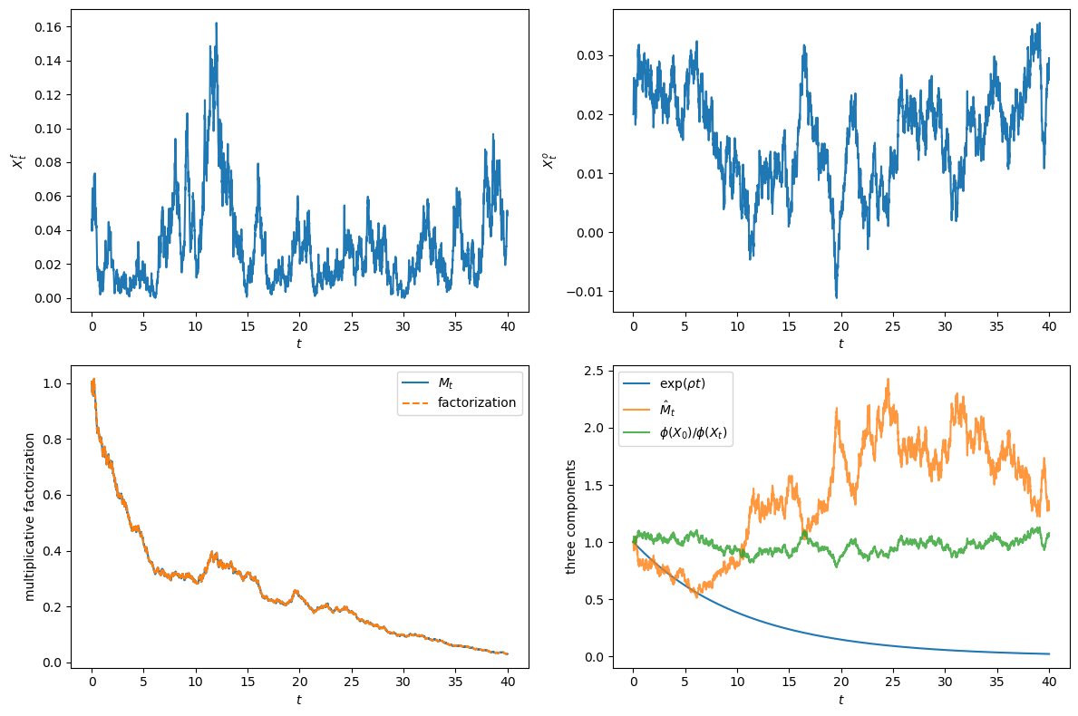
Fig. 104.3 Affine state paths and multiplicative factorization#
The figure shows how the three components evolve over time.
104.8. Long-run risk prices#
We can now use the factorization to compute long-run analogues of the instantaneous risk prices that arise in standard continuous-time asset pricing.
We can ask:
If an investor takes on a small exposure to a shock today, how much extra expected return do they need when that return is measured as a long-horizon rate rather than an instantaneous one?
The two answers, local and long-run, need not agree.
A shock that moves a persistent state variable has a small immediate effect on the cash flow but a large cumulative effect on future expected growth and discounting, which is why the two answers come apart.
So the long-run risk price is the local price plus a persistence correction.
The size of the correction depends on the speed of mean reversion.
104.8.1. Defining the prices#
Definition 104.19 (Local Brownian Risk Price)
The local Brownian risk price is the state-dependent vector \(-\gamma^s(x)\).
A small Brownian exposure \(\gamma^v_i\) earns a required expected return of \(-\gamma^v_i \gamma^s_i\) per unit time, so a unit of exposure \(\gamma^v_i\) is priced at \(-\gamma^s_i\).
For the local price we just read off the SDF coefficients.
Definition 104.20 (Long-Run Risk Price)
The long-run risk price is the marginal change in the long-run required return on a cash flow with respect to a small change in its risk exposure.
When we work with growing cash flows, the long-run required return is \(R_\infty = -\rho + \delta\), where \(\rho\) is the principal eigenvalue of the \(GS\) semigroup and \(\delta\) is the trend growth rate, held fixed.
Computing the long-run price requires solving the principal eigenvalue problem, which captures how a shock propagates through the persistent state component.
104.8.2. Two frontiers#
We will see two related ways to vary risk exposure, each leading to a slightly different long-run risk price:
Valuation-functional frontier:
Hold the SDF \(S\) fixed and vary the asset’s Brownian exposures \((\gamma^v_f, \gamma^v_o)\).
Use the local pricing restriction to determine the drift \(\beta^v\), then compute \(\rho^v\) for the \(V\)-semigroup.
Cash-flow frontier:
Hold the SDF \(S\) fixed and vary the cash-flow’s growth exposures \((\gamma^g_f, \gamma^g_o)\).
Set \(M = GS\) and compute the principal eigenvalue \(\rho\) of the cash-flow valuation semigroup.
These two frontiers coincide in simple log-normal examples, but they can differ with stochastic volatility, nonlinear dynamics, or jump risk.
We will work out both in the affine model below.
104.8.3. Stochastic discount factor decomposition#
Before getting into risk prices, a natural benchmark is the case \(M=S\): applying the factorization (104.1) directly to the SDF itself.
The factorization becomes
This is the permanent-transitory decomposition of Alvarez and Jermann [2005], now linked to a concrete eigenfunction construction.
The factor \(\exp(\rho t)\) is the deterministic trend in the SDF and the martingale \(\hat M\) is its random permanent component; the state-dependent ratio is transient and washes out.
See also
The same spectral decomposition of the pricing operator is the central tool in The Recovery Theorem, which uses it to “recover” subjective beliefs from observed prices, and in Misspecified recovery, which examines what goes wrong when the permanent martingale component is mistakenly assumed away.
For a long zero-coupon bond,
so long-maturity discount bond prices depend on the current state primarily through the eigenfunction \(\phi\).
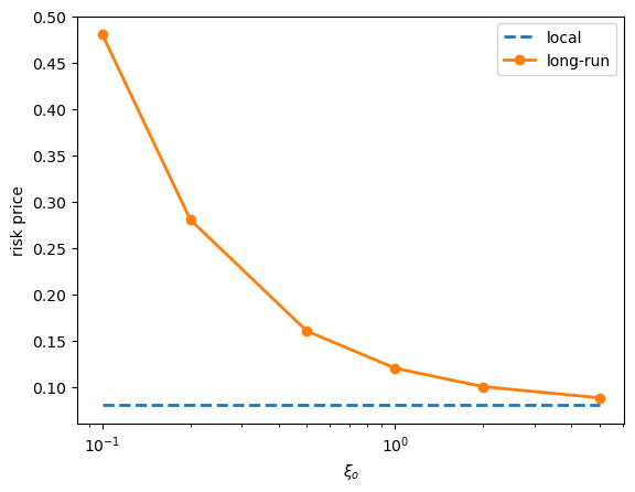
104.8.4. Comparison in the affine model#
For the affine specification, we can write closed-form expressions for both local and long-run prices of a \(B^o\) shock.
The local price is just
The long-run price (which we will derive below using the valuation-functional frontier) is
The extra term \(-(\beta_o^s/\xi_o)\sigma_o\) is the persistence correction.
It arises because:
a \(B^o\) shock moves the persistent growth predictor \(X^o\), and
\(X^o\) mean reverts at rate \(\xi_o\), so the cumulative effect of the shock on future SDF growth scales like \(1/\xi_o\).
As \(\xi_o\) shrinks, persistence grows and the long-run price diverges from the local one, which is the central economic content of long-run risk models.
The local price of \(B^f\) exposure is state dependent (it scales with \(\sqrt{X^f_t}\)), and the long-run price of \(B^f\) exposure is nonlinear, since \(c_f\) is the root of a quadratic.
γ_s_o = params_sdf["γ_o"]
β_s_o = params_sdf["β_o"]
ξ_o = params_sdf["ξ_o"]
σ_o = params_sdf["σ_o"]

local_price_o = -γ_s_o
long_run_price_o = -γ_s_o - (β_s_o / ξ_o) * σ_o

print(f"local price of B^o exposure    = {local_price_o:.4f}")
print(f"long-run price of B^o exposure = {long_run_price_o:.4f}")
local price of B^o exposure    = 0.0800
long-run price of B^o exposure = 0.1600
The next cell illustrates how persistence changes the wedge between local and long-run prices.
ξ_o_grid = np.array([0.10, 0.20, 0.50, 1.00, 2.00, 5.00])
local_grid = np.full_like(ξ_o_grid, local_price_o)
long_grid = -γ_s_o - (β_s_o / ξ_o_grid) * σ_o

fig, ax = plt.subplots()
ax.plot(ξ_o_grid, local_grid, "--", lw=2, label="local")
ax.plot(ξ_o_grid, long_grid, "o-", lw=2, label="long-run")
ax.set_xscale("log")
ax.set_xlabel("mean-reversion speed $\\xi_o$")
ax.set_ylabel("risk price")
ax.legend()
plt.show()
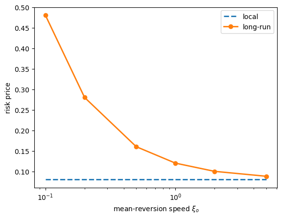
Fig. 104.4 Persistence and long-run risk prices#
As we can see, the long-run price of \(B^o\) exposure is sensitive to the mean-reversion speed \(\xi_o\), but the local price is a constant.
104.8.5. Changing valuation functionals#
Now we work out the long-run risk price formula by varying the asset’s exposure, the valuation-functional frontier introduced above.
We hold the SDF \(S\) fixed and pick Brownian exposures \((\gamma_f^v,\gamma_o^v)\) for the asset return, parameterizing the valuation functional as
The martingale restriction on \(VS\) determines the drift coefficients from the chosen Brownian exposures \((\gamma_f^v,\gamma_o^v)\):
Applying the affine eigenvalue formula to \(M=V\) gives
where \(c_o^v=\beta_o^v/\xi_o=-\beta_o^s/\xi_o\) and \(c_f^v\) solves the same quadratic equation as in (104.16) with \((\beta_f,\gamma_f)\) replaced by \((\beta_f^v,\gamma_f^v)\).
Holding \(\gamma_f^v\) fixed, differentiating (104.27) with respect to \(\gamma_o^v\) gives the long-run valuation-functional price of \(B^o\) exposure:
This matches the formula (104.25) we previewed above, namely the local price plus the persistence correction \(-(\beta_o^s/\xi_o)\sigma_o\).
Let’s verify the formula numerically by finite-differencing the eigenvalue computation.
def valuation_params_from_exposure(γ_v_o, γ_v_f=0.0):
    """Affine parameters for a valuation functional V."""
    p = dict(params_sdf)
    p.update({
        "β_bar": (-params_sdf["β_bar"]
                  - 0.5 * (params_sdf["γ_o"] + γ_v_o) ** 2),
        "β_f": (-params_sdf["β_f"]
                - 0.5 * (params_sdf["γ_f"] + γ_v_f) ** 2),
        "β_o": -params_sdf["β_o"],
        "γ_f": γ_v_f,
        "γ_o": γ_v_o,
    })
    return p


def valuation_eigenvalue_for_exposure(γ_v_o, γ_v_f=0.0):
    """Principal eigenvalue for the valuation functional frontier."""
    p = valuation_params_from_exposure(γ_v_o, γ_v_f)
    _, _, ρ, _ = solve_affine_eigenfunction(p)
    return ρ
γ_v_o_grid = np.linspace(-0.5, 0.5, 101)
ρ_v_grid = np.array([
    valuation_eigenvalue_for_exposure(g) for g in γ_v_o_grid
])

fig, ax = plt.subplots()
ax.plot(γ_v_o_grid, ρ_v_grid, lw=2)
ax.set_xlabel("valuation exposure $\\gamma_o^v$")
ax.set_ylabel("principal eigenvalue $\\rho^v$")
plt.show()
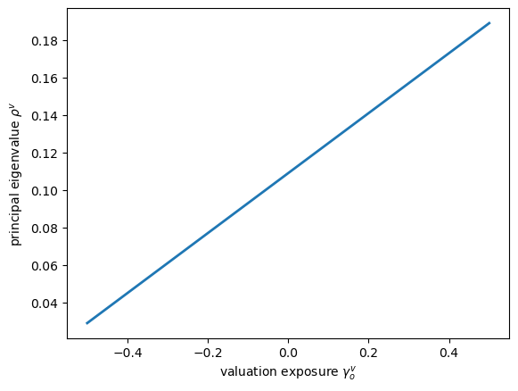
Fig. 104.5 Changing valuation functionals#
valuation_slope = (
    valuation_eigenvalue_for_exposure(0.001)
    - valuation_eigenvalue_for_exposure(-0.001)
) / 0.002

print(f"finite-difference slope = {valuation_slope:.6f}")
print(f"formula                 = {long_run_price_o:.6f}")
finite-difference slope = 0.160000
formula                 = 0.160000
104.8.6. Changing cash-flow risk#
The second long-run frontier varies the cash-flow’s exposure to risk rather than the return.
We pick a growth functional \(G_t = \exp(A_t^g)\) with the affine parameterization
The last line is the Itô compensator that makes \(\exp(A_t^g-\delta t) = \hat G_t\) a local martingale, with \(\delta\) the constant trend growth rate.
Stochastic stability of the growth-twisted process needs three conditions.
The Feller-type nonattainment inequality
keeps the twisted \(X^f\) from hitting zero.
Mean reversion of the twisted \(X^f\) is picked by the same root-selection argument we used for the SDF in (104.18).
\(\hat G\) itself must be a martingale, the Assumption-6.1 analogue for the growth twist.
The Feller inequality is necessary but not sufficient on its own.
Note
This Feller restriction is a concrete instance of a general point we flagged earlier: changing growth risk can violate stability and invalidate the long-run approximation, so the choice of \((\gamma_f^g, \gamma_o^g)\) isn’t free.
To price the cash flow \(D_t=D_0G_t\psi(X_t)\), use the semigroup generated by \(M=GS\).
The combined affine parameters are
Let \(\rho\) be the principal eigenvalue of this \(GS\) semigroup.
Then \(-\rho\) is the long-run decay rate in value, and
is the asymptotic required return net of the cash-flow growth rate.
def required_return_for_growth_exposure(γ_g_o, γ_g_f=0.0, δ=0.02):
    """Long-run required return for a cash-flow growth exposure."""
    p = dict(params_sdf)
    p.update({
        "β_bar": params_sdf["β_bar"] + δ - 0.5 * γ_g_o ** 2,
        "β_f": params_sdf["β_f"] - 0.5 * γ_g_f ** 2,
        "β_o": params_sdf["β_o"],
        "γ_f": params_sdf["γ_f"] + γ_g_f,
        "γ_o": params_sdf["γ_o"] + γ_g_o,
    })

    _, _, ρ, _ = solve_affine_eigenfunction(p)
    return -ρ + δ
γ_g_o_grid = np.linspace(-0.5, 0.5, 101)
required_returns = np.array([
    required_return_for_growth_exposure(g) for g in γ_g_o_grid
])

local_line = (required_return_for_growth_exposure(0.0)
              + local_price_o * γ_g_o_grid)

fig, ax = plt.subplots()
ax.plot(γ_g_o_grid, required_returns, lw=2,
        label="long-run required return")
ax.plot(γ_g_o_grid, local_line, "--", lw=2,
        label="local slope")
ax.set_xlabel("cash-flow exposure $\\gamma_o^g$")
ax.set_ylabel("rate of return")
ax.legend()
plt.show()
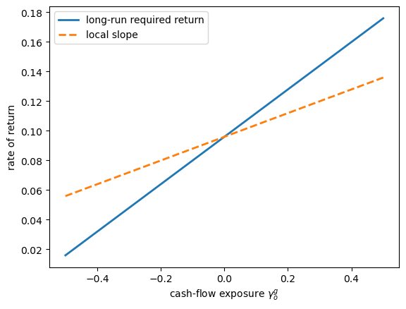
Fig. 104.6 Local and long-run pricing of persistent growth risk#
The slope of the long-run line is the risk price in (104.25), and the dashed line shares the same value at \(\gamma_o^g = 0\) but with slope equal to the local Brownian risk price \(-\gamma_o^s\).
The gap between the two slopes is the persistence correction; the dashed line is a slope comparator, not the actual Breeden local expected-return frontier (which is state dependent in \(X^f\) and \(X^o\)).
finite_difference = (
    required_return_for_growth_exposure(0.001)
    - required_return_for_growth_exposure(-0.001)
) / 0.002

print(f"finite-difference slope = {finite_difference:.6f}")
print(f"formula                 = {long_run_price_o:.6f}")
finite-difference slope = 0.160000
formula                 = 0.160000
104.9. Assumptions behind the scenes#
The examples above make the eigenfunction calculation look routine.
For finite-state chains and the affine model, it really is; Perron-Frobenius theory and closed-form algebra handle every requirement.
But in a general state space, three things can go wrong, each corresponding to one of the assumptions we have been carrying.
The rest of this section examines each in turn.
104.9.1. Issue 1: \(\hat M\) might fail to be a martingale#
A positive eigenfunction \(\phi\) gives us a candidate martingale \(\hat M\) from (104.10), but \(\hat M\) is only a nonnegative local martingale, hence a supermartingale.
A supermartingale is not enough to define a probability measure: we need \(\mathbb{E}[\hat M_t] = 1\), i.e. a genuine martingale, the content of Assumption 6.1 in Hansen and Scheinkman [2009].
A standard way to verify this is a two-sided Girsanov construction: write the drift and jump distortion induced by \(\hat M\), check that the distorted Markov process is well-behaved, and verify that the reverse density (the inverse of \(\hat M\)) is locally integrable.
104.9.2. Issue 2: the twisted process might fail to be stable#
Even with \(\hat M\) a martingale, the long-run limit (104.12) requires that the twisted process actually settles into a steady state.
This is where stochastic stability (our trio of stationary distribution, irreducibility of the skeleton, and Harris recurrence) does real work.
The affine example illustrates this concretely, since we rejected one of the two algebraically valid eigenfunctions because it implied an explosive twisted square-root process.
104.9.3. Issue 3: a principal eigenfunction might not exist at all#
In a general state space, even existence of a strictly positive eigenfunction is not automatic.
A standard sufficient condition starts with a Lyapunov-type drift bound: there is a function \(V \geq 1\) on the state space and a constant \(a_0\) such that
Roughly: \(V\) doesn’t grow too fast under the semigroup.
With this in hand, for any \(\alpha > a_0\) define the resolvent operator
\(F_\alpha\) is the Laplace transform of the semigroup generated by the rescaled multiplicative functional \(M_t V(X_t)/V(X_0)\).
The existence proof then proceeds in three steps:
Irreducibility for the resolvent. There exists a reference measure \(\nu\) such that \(F_\alpha\mathbf 1_\Lambda(x) > 0\) for every \(x\) whenever \(\nu(\Lambda) > 0\), so the resolvent doesn’t “miss” any region of state space.
Nummelin minorization. Irreducibility yields a bounded nonnegative function \(s\) on the state space, with \(\int s\, d\nu > 0\), such that for every nonnegative \(\psi\),
\[ F_\alpha \psi(x)\, \geq\, s(x) \int \psi\, d\nu . \]The function \(s\) (often called the minorization function) measures how strongly the resolvent dominates a fixed reference measure \(\nu\).
Eigenfunction extraction. The minorization, combined with additional boundedness or strengthened drift assumptions, identifies a critical spectral value for \(F_\alpha\) and an associated positive eigenfunction.
Inverting the resolvent transform produces a positive eigenfunction for the original semigroup.
These steps are all nontrivial and are out of scope for this lecture.
The details are in Section 9 of Hansen and Scheinkman [2009].
We can summarize the chain of conditions as:
Want |
Need |
|---|---|
A factorization (104.1) |
A positive eigenfunction \(\phi\) |
\(\hat M\) to define a probability measure |
\(\hat M\) is a martingale (Assumption 6.1) |
The long-run limit (104.12) |
Stochastic stability of the twisted process |
A unique principal eigenfunction |
Stability selects among positive eigenfunctions |
In the finite-state case, all four follow from one Perron-Frobenius calculation; in the affine model, they reduce to picking the right root of a quadratic. In general, each must be checked separately.
The full theory in Hansen and Scheinkman [2009] also delivers stronger \(L^p\) approximation results and Lyapunov criteria for stochastic stability, which we don’t reproduce here.
104.10. Summary#
The Hansen-Scheinkman approach studies long-run risk by studying positive eigenfunctions of valuation semigroups.
The main steps are:
Model discounting, growth, or cumulated returns by a positive multiplicative functional \(M\).
Build the semigroup \(\mathbb M_t\psi(x)=\mathbb{E}[M_t\psi(X_t)\mid X_0=x]\).
When \(M = VS\) is the product of a valuation functional and an SDF, impose the local pricing restriction that \(VS\) is a martingale; for cash-flow valuation semigroups \(\mathbb Q_t = GS\), the pricing restriction is on \(S\) alone, and \(G\) enters only as a growth twist.
Solve the principal eigenvalue problem \(\mathbb A\phi=\rho\phi\).
Use the factorization \(M_t=\exp(\rho t)\hat M_t\phi(X_0)/\phi(X_t)\).
Under the twisted probability measure induced by \(\hat M\), use stability to obtain long-run approximations of the form (104.12).
In finite-state problems, this is Perron-Frobenius theory.
In affine diffusion problems, exponential-affine eigenfunctions often produce closed-form formulas.
The long-run risk prices that emerge can differ sharply from local risk prices when shocks move persistent state variables.
This persistence effect is the economic channel emphasized in long-run risk asset-pricing models and in the empirical work of Hansen et al. [2008].
104.11. Exercises#
Exercise 104.1
Consider a two-state Markov chain with intensity matrix
Let the multiplicative functional have decay rate \(r_1>0\) in state 1, decay rate \(r_2=0\) in state 2, and no jumps.
Write down the generator matrix \(A\).
Find the principal eigenvalue \(\rho\) in terms of \(\lambda\), \(\mu\), and \(r_1\).
Verify numerically with \(\lambda=0.4\), \(\mu=0.6\), and \(r_1=0.05\).
Show that \(-r_1 < \rho < 0\).
Solution
Here is one solution:
1. The generator is
2. The characteristic equation is
Hence the principal eigenvalue is the larger root
3. Numerical verification:
λ, μ, r1 = 0.4, 0.6, 0.05

disc = (λ + μ + r1) ** 2 - 4 * μ * r1
ρ_formula = (-(λ + μ + r1) + np.sqrt(disc)) / 2

U_ex = np.array([[-λ, λ],
                 [μ, -μ]])
r_ex = np.array([r1, 0.0])
κ_ex = np.zeros((2, 2))

A_ex = build_generator(U_ex, r_ex, κ_ex)
ρ_numeric, φ_numeric = principal_eigenpair(A_ex)

print(f"formula  ρ = {ρ_formula:.8f}")
print(f"numeric  ρ = {ρ_numeric:.8f}")
print(f"difference   = {abs(ρ_formula-ρ_numeric):.2e}")
formula  ρ = -0.02939431
numeric  ρ = -0.02939431
difference   = 0.00e+00
4. Let
Then \(q(0)=\mu r_1>0\) and
Since the parabola opens upward, one root lies in \((-r_1,0)\).
The principal eigenvalue is the larger root, so \(-r_1<\rho<0\).
Exercise 104.2
In the affine model, compute the local and long-run prices of exposure to \(B^o\) for
Use the formulas
and
Explain why the two prices converge as \(\xi_o \to \infty\).
Solution
Here is one solution:
ξ_vals = np.array([0.1, 0.2, 0.5, 1.0, 2.0, 5.0])
local_vals = np.full_like(ξ_vals, -params_sdf["γ_o"])
long_vals = (-params_sdf["γ_o"]
             - (params_sdf["β_o"] / ξ_vals) * params_sdf["σ_o"])

for ξ, lp, lrp in zip(ξ_vals, local_vals, long_vals):
    print(f"ξ_o = {ξ:3.1f}: local = {lp:.4f}, long-run = {lrp:.4f}")

fig, ax = plt.subplots()
ax.plot(ξ_vals, local_vals, "--", lw=2, label="local")
ax.plot(ξ_vals, long_vals, "o-", lw=2, label="long-run")
ax.set_xscale("log")
ax.set_xlabel("$\\xi_o$")
ax.set_ylabel("risk price")
ax.legend()
plt.show()
ξ_o = 0.1: local = 0.0800, long-run = 0.4800
ξ_o = 0.2: local = 0.0800, long-run = 0.2800
ξ_o = 0.5: local = 0.0800, long-run = 0.1600
ξ_o = 1.0: local = 0.0800, long-run = 0.1200
ξ_o = 2.0: local = 0.0800, long-run = 0.1000
ξ_o = 5.0: local = 0.0800, long-run = 0.0880
As \(\xi_o\) increases, \(X^o\) mean reverts faster.
A shock to \(B^o\) then has a shorter-lived effect on future expected growth.
The persistence term \((\beta_o^s/\xi_o)\sigma_o\) converges to zero, so the long-run price converges to the local price.
Exercise 104.3
Consider a three-state chain with states {expansion, normal, contraction}, intensity matrix
decay-rate vector \(r = (0.06, 0.04, 0.01)\), and no jumps in the multiplicative functional. Let \(\psi=(3,1,2)\).
Compute the principal eigenpair \((\rho,\phi)\) and twisted stationary distribution \(\hat\varsigma\), and report the theoretical limit
Plot
on a logarithmic scale.
Compare the convergence rate to the spectral gap between the largest and second-largest real parts of the eigenvalues of \(A\).
Solution
Here is one solution:
state_names = ["expansion", "normal", "contraction"]

U3 = np.array([[-0.40,  0.30,  0.10],
               [ 0.20, -0.50,  0.30],
               [ 0.10,  0.20, -0.30]])

r3 = np.array([0.06, 0.04, 0.01])
κ3 = np.zeros((3, 3))

A3 = build_generator(U3, r3, κ3)
ρ3, φ3 = principal_eigenpair(A3)
A3_hat = twisted_generator(A3, ρ3, φ3)
ς3 = stationary_distribution(A3_hat)

ψ = np.array([3.0, 1.0, 2.0])
limit = φ3 * np.sum((ψ / φ3) * ς3)

print("limit:")
for name, value in zip(state_names, limit):
    print(f"  {name:11s} {value:.6f}")

t_vals = np.linspace(0.1, 40, 300)
errors = np.array([
    np.max(np.abs(np.exp(-ρ3 * t_val) * expm(t_val * A3) @ ψ - limit))
    for t_val in t_vals
])

eigenvalues = eig(A3, right=False)
real_parts = np.sort(eigenvalues.real)[::-1]
gap = real_parts[0] - real_parts[1]

fig, ax = plt.subplots()
ax.semilogy(t_vals, errors, lw=2)
ax.set_xlabel("$t$")
ax.set_ylabel("error")
plt.show()

print(f"spectral gap = {gap:.6f}")
limit:
  expansion   1.808490
  normal      1.906080
  contraction 2.021897
spectral gap = 0.462679
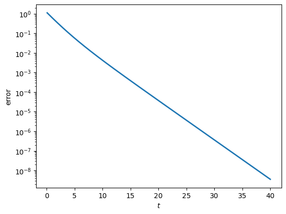
The normalized semigroup converges at an exponential rate governed by the separation between the dominant eigenvalue and the remaining eigenvalues.
In this finite-state example, that separation is the spectral gap computed above.
Exercise 104.4
Derive the local martingale restriction (104.5) from Itô’s formula.
Let \(M = \exp(A)\) for the additive functional \(A\) in (104.3), with parameters \((\beta,\gamma,\kappa)\).
Decompose \(A_t = A_t^c + A_t^j\) into its continuous and pure-jump parts and write down \(dA_t^c\) and the jump magnitudes \(\Delta A_t\).
Apply Itô’s formula for semimartingales to \(f(a) = e^a\) to show that
Use \(d\langle A^c, A^c\rangle_t = \gamma^\top\gamma\, dt\) and rewrite the jump term as an integral against the random counting measure \(\zeta\).
Split \(\zeta\) into its compensator \(\eta(dy \mid X_{t-})\, dt\) and the compensated martingale measure \(\tilde\zeta = \zeta - \eta(dy\mid X_{t-})\, dt\).
Collect drift (predictable) and martingale terms and conclude that \(M\) is a local martingale iff the drift vanishes at every state, which gives (104.5).
Solution
Here is one solution.
1. From the parameterization (104.3),
2. For \(f(a) = e^a\) we have \(f'(a) = f''(a) = e^a\), so \(f'(A_{t-}) = f''(A_{t-}) = M_{t-}\).
The (generalized) Itô’s formula for a semimartingale gives
Since \(A_t = A_{t-} + \Delta A_t\) at a jump, \(f(A_t) - f(A_{t-}) = M_{t-}\big(\exp[\Delta A_t] - 1\big)\), which is the stated expression.
3. Substituting \(d\langle A^c, A^c\rangle_t = \gamma(X_{t-})^\top \gamma(X_{t-})\, dt\) and rewriting the jump contribution as an integral against the random counting measure \(\zeta\) of \((X, A)\) gives
4. Writing \(\zeta = \tilde\zeta + \eta(dy\mid X_{t-})\, dt\) separates the jump integral into a martingale and a predictable drift contribution:
5. Collecting drift and martingale terms,
The Brownian and compensated-jump terms are local martingales, so \(M\) is a local martingale iff the bracketed drift vanishes for every state \(x\), giving (104.5).
Exercise 104.5
Derive the closed-form expression for the extended generator in (104.8).
Take the jump-diffusion setting in which the Markov state satisfies
between jumps, with \(\Sigma = \Gamma\Gamma^\top\) and jump compensator \(\eta(dy \mid x)\).
Let \(M = \exp(A)\) for the additive functional \(A\) in (104.3) and let \(\phi\) be a smooth, strictly positive function.
Recall from Definition 104.10 that \(\mathbb A\phi = \chi\) if
is a local martingale. The task therefore has two pieces: identify the predictable drift of \(M_t\phi(X_t)\) to read off a candidate \(\chi\), and verify that the residual \(N_t\) really is a local martingale.
(1) Apply Itô’s formula to \(Y_t = \exp(A_t)\phi(X_t)\) between jumps and show that the continuous part of \(dY_t\) has drift
(2) Show that at a jump time \(t\) with \(X_{t-}=x\) and \(X_t=y\),
and conclude that the predictable jump compensator contributes drift
(3) Decompose
combine with part (1) to obtain the full predictable drift coefficient \(\chi(x)\), and check that it matches the closed form (104.8).
(4) Identify the continuous Itô integrand from part (1) as a local martingale \(N^c_t\) and the compensated jump sum from part (2) as a local martingale \(N^j_t\).
Show that the semimartingale decomposition of \(Y_t = M_t\phi(X_t)\) implies
which is a local martingale. Conclude via Definition 104.10 that \(\mathbb A \phi = \chi\).
Solution
Here is one solution:
(1) Set \(g(a, x) = e^a \phi(x)\), so that \(Y_t = g(A_t, X_t)\).
Between jumps, the continuous parts of \(A\) and \(X\) are
with quadratic covariations
The partial derivatives of \(g\) satisfy
Itô’s formula yields a continuous local martingale \(N^c_t\) (the \(dB_t\) part) plus the drift
Grouping the gradient terms gives the expression in the question.
(2) At a jump time \(t\), \(\Delta A_t = \kappa(X_t, X_{t-}) = \kappa(y, x)\), so \(M_t = M_{t-}\exp[\kappa(y,x)]\) and
The sum of jumps minus its predictable compensator is a local martingale \(N^j_t\), and the compensator itself contributes the predictable drift quoted in the question.
(3) Adding the jump drift from (2) to the continuous drift from (1), the predictable drift of \(Y_t = M_t \phi(X_t)\) at state \(x\) is \(M_t\, \chi(x)\, dt\) with
Collecting the terms multiplying \(\phi(x)\) recovers (104.8).
(4) Putting the two martingale pieces together and integrating the drift, steps (1) and (2) give the semimartingale decomposition
Rearranging,
which is a local martingale because it is a sum of local martingales.
This is exactly the property required by Definition 104.10, so \(\chi = \mathbb A \phi\).